Spectral Theory 谱理论
本页译自 LibreTexts · A First Course in Linear Algebra (Kuttler)「Spectral Theory(谱理论)」第 7 章各节及习题。公式经 MathJax 渲染,自定义宏已注入;正文与译文段段对照。
Outcomes 学习目标
- Describe eigenvalues geometrically and algebraically.
- Find eigenvalues and eigenvectors for a square matrix.
- 用几何与代数两种方式描述特征值。
- 求方阵的特征值与特征向量。
Spectral Theory refers to the study of eigenvalues and eigenvectors of a matrix. It is of fundamental importance in many areas and is the subject of our study for this chapter.
Definition of Eigenvectors and Eigenvalues 特征值与特征向量的定义
In this section, we will work with the entire set of complex numbers, denoted by $\mathbb{C}$. Recall that the real numbers, $\mathbb{R}$ are contained in the complex numbers, so the discussions in this section apply to both real and complex numbers.
To illustrate the idea behind what will be discussed, consider the following example.
Example 1: Eigenvectors and Eigenvalues 例 1:特征值与特征向量
Let $A = \left[ \begin{array}{rrr} 0 & 5 & -10 \\ 0 & 22 & 16 \\ 0 & -9 & -2 \end{array} \right]$ Compute the product $AX$ for $X = \left[ \begin{array}{r} -5 \\ -4 \\ 3 \end{array} \right], X = \left[ \begin{array}{r} 1 \\ 0 \\ 0 \end{array} \right]$ What do you notice about $AX$ in each of these products?
Solution 解
First, compute $AX$ for $X =\left[ \begin{array}{r} -5 \\ -4 \\ 3 \end{array} \right]$
This product is given by $AX = \left[ \begin{array}{rrr} 0 & 5 & -10 \\ 0 & 22 & 16 \\ 0 & -9 & -2 \end{array} \right] \left[ \begin{array}{r} -5 \\ -4 \\ 3 \end{array} \right] = \left[ \begin{array}{r} -50 \\ -40 \\ 30 \end{array} \right] =10\left[ \begin{array}{r} -5 \\ -4 \\ 3 \end{array} \right]$
In this case, the product $AX$ resulted in a vector which is equal to $10$ times the vector $X$. In other words, $AX=10X$.
Let’s see what happens in the next product. Compute $AX$ for the vector $X = \left[ \begin{array}{r} 1 \\ 0 \\ 0 \end{array} \right]$
This product is given by $AX = \left[ \begin{array}{rrr} 0 & 5 & -10 \\ 0 & 22 & 16 \\ 0 & -9 & -2 \end{array} \right] \left[ \begin{array}{r} 1 \\ 0 \\ 0 \end{array} \right] = \left[ \begin{array}{r} 0 \\ 0 \\ 0 \end{array} \right] =0\left[ \begin{array}{r} 1 \\ 0 \\ 0 \end{array} \right]$
In this case, the product $AX$ resulted in a vector equal to $0$ times the vector $X$, $AX=0X$.
Perhaps this matrix is such that $AX$ results in $kX$, for every vector $X$. However, consider $\left[ \begin{array}{rrr} 0 & 5 & -10 \\ 0 & 22 & 16 \\ 0 & -9 & -2 \end{array} \right] \left[ \begin{array}{r} 1 \\ 1 \\ 1 \end{array} \right] = \left[ \begin{array}{r} -5 \\ 38 \\ -11 \end{array} \right] $ In this case, $AX$ did not result in a vector of the form $kX$ for some scalar $k$.
There is something special about the first two products calculated in Example PageIndex 1. Notice that for each, $AX=kX$ where $k$ is some scalar. When this equation holds for some $X$ and $k$, we call the scalar $k$ an eigenvalue of $A$. We often use the special symbol $\lambda$ instead of $k$ when referring to eigenvalues. In Example PageIndex 1, the values $10$ and $0$ are eigenvalues for the matrix $A$ and we can label these as $\lambda_1 = 10$ and $\lambda_2 = 0$.
When $AX = \lambda X$ for some $X \neq 0$, we call such an $X$ an eigenvector of the matrix $A$. The eigenvectors of $A$ are associated to an eigenvalue. Hence, if $\lambda_1$ is an eigenvalue of $A$ and $AX = \lambda_1 X$, we can label this eigenvector as $X_1$. Note again that in order to be an eigenvector, $X$ must be nonzero.
There is also a geometric significance to eigenvectors. When you have a nonzero vector which, when multiplied by a matrix results in another vector which is parallel to the first or equal to 0, this vector is called an eigenvector of the matrix. This is the meaning when the vectors are in $\mathbb{R}^{n}.$
The formal definition of eigenvalues and eigenvectors is as follows.
Definition 1: Eigenvalues and Eigenvectors 定义 1:特征值与特征向量
Let $A$ be an $n\times n$ matrix and let $X \in \mathbb{C}^{n}$ be a nonzero vector for which
$AX=\lambda X$ for some scalar $\lambda .$ Then $\lambda$ is called an eigenvalue of the matrix $A$ and $X$ is called an eigenvector of $A$ associated with $\lambda$, or a $\lambda$-eigenvector of $A$.
The set of all eigenvalues of an $n\times n$ matrix $A$ is denoted by $\sigma \left( A\right)$ and is referred to as the spectrum of $A.$
The eigenvectors of a matrix $A$ are those vectors $X$ for which multiplication by $A$ results in a vector in the same direction or opposite direction to $X$. Since the zero vector $0$ has no direction this would make no sense for the zero vector. As noted above, $0$ is never allowed to be an eigenvector.
Let’s look at eigenvectors in more detail. Suppose $X$ satisfies 上述等式. Then $\begin{array}{c} AX - \lambda X = 0 \\ \mbox{or} \\ \left( A-\lambda I\right) X = 0 \end{array}$ for some $X \neq 0.$ Equivalently you could write $\left( \lambda I-A\right)X = 0$, which is more commonly used. Hence, when we are looking for eigenvectors, we are looking for nontrivial solutions to this homogeneous system of equations!
Recall that the solutions to a homogeneous system of equations consist of basic solutions, and the linear combinations of those basic solutions. In this context, we call the basic solutions of the equation $\left( \lambda I - A\right) X = 0$ basic eigenvectors. It follows that any (nonzero) linear combination of basic vectors is again an eigenvector.
Suppose the matrix $\left(\lambda I - A\right)$ is invertible, so that $\left(\lambda I - A\right)^{-1}$ exists. Then the following equation would be true. $\begin{aligned} X &= IX \\ &= \left( \left( \lambda I - A\right) ^{-1}\left(\lambda I - A \right) \right) X \\ &=\left( \lambda I - A\right) ^{-1}\left( \left( \lambda I - A\right) X\right) \\ &= \left( \lambda I - A\right) ^{-1}0 \\ &= 0\end{aligned}$ This claims that $X=0$. However, we have required that $X \neq 0$. Therefore $\left(\lambda I - A\right)$ cannot have an inverse!
Recall that if a matrix is not invertible, then its determinant is equal to $0$. Therefore we can conclude that $\det \left( \lambda I - A\right) =0$ Note that this is equivalent to $\det \left(A- \lambda I \right) =0$.
The expression $\det \left( \lambda I-A\right)$ is a polynomial (in the variable $x\$ called the characteristic polynomial of $A$, and $\det \left( \lambda I-A\right) =0$ is called the characteristic equation. For this reason we may also refer to the eigenvalues of $A$ as characteristic values, but the former is often used for historical reasons.$
The following theorem claims that the roots of the characteristic polynomial are the eigenvalues of $A$. Thus when 上述等式 holds, $A$ has a nonzero eigenvector.
Theorem 1: The Existence of an Eigenvector 定理 1:特征向量的存在性
Let $A$ be an $n\times n$ matrix and suppose $\det \left( \lambda I - A\right) =0$ for some $\lambda \in \mathbb{C}$.
Then $\lambda$ is an eigenvalue of $A$ and thus there exists a nonzero vector $X \in \mathbb{C}^{n}$ such that $AX=\lambda X$.
Proof. For $A$ an $n\times n$ matrix, the method of Laplace Expansion demonstrates that $\det \left( \lambda I - A \right)$ is a polynomial of degree $n.$ As such, the equation 上述等式 has a solution $\lambda \in \mathbb{C}$ by the Fundamental Theorem of Algebra. The fact that $\lambda$ is an eigenvalue is left as an exercise.
Finding Eigenvectors and Eigenvalues 求特征向量与特征值
Now that eigenvalues and eigenvectors have been defined, we will study how to find them for a matrix $A$.
First, consider the following definition.
Definition 2: Multiplicity of an Eigenvalue 定义 2:特征值的重数
Let $A$ be an $n \times n$ matrix with characteristic polynomial given by $\det \left( \lambda I - A\right)$. Then, the multiplicity of an eigenvalue $\lambda$ of $A$ is the number of times $\lambda$ occurs as a root of that characteristic polynomial.
For example, suppose the characteristic polynomial of $A$ is given by $\left( \lambda - 2 \right)^2$. Solving for the roots of this polynomial, we set $\left( \lambda - 2 \right)^2 = 0$ and solve for $\lambda $. We find that $\lambda = 2$ is a root that occurs twice. Hence, in this case, $\lambda = 2$ is an eigenvalue of $A$ of multiplicity equal to $2$.
We will now look at how to find the eigenvalues and eigenvectors for a matrix $A$ in detail. The steps used are summarized in the following procedure.
Procedure 1: Finding Eigenvalues and Eigenvectors 步骤 1:求特征值与特征向量
Let $A$ be an $n \times n$ matrix.
- First, find the eigenvalues $\lambda$ of $A$ by solving the equation $\det \left( \lambda I -A \right) = 0$.
- For each $\lambda$, find the basic eigenvectors $X \neq 0$ by finding the basic solutions to $\left( \lambda I - A \right) X = 0$.
- 首先,通过解方程 $\det \left( \lambda I -A \right) = 0$ 求出 $A$ 的特征值 $\lambda$。
- 对每个 $\lambda$,求 $\left( \lambda I - A \right) X = 0$ 的基本解,即得到基本特征向量 $X \neq 0$。
To verify your work, make sure that $AX=\lambda X$ for each $\lambda$ and associated eigenvector $X$.
We will explore these steps further in the following example.
Example 2: Find the Eigenvalues and Eigenvectors 例 2:求特征值与特征向量
Let $A = \left[ \begin{array}{rr} -5 & 2 \\ -7 & 4 \end{array} \right]$. Find its eigenvalues and eigenvectors.$
Solution 解
We will use Procedure PageIndex 1. First we find the eigenvalues of $A$ by solving the equation $\det \left( \lambda I - A \right) =0 $
This gives $\begin{aligned} \det \left( \lambda \left[ \begin{array}{rr} 1 & 0 \\ 0 & 1 \end{array} \right] - \left[ \begin{array}{rr} -5 & 2 \\ -7 & 4 \end{array} \right] \right) &= 0 $ $ \det \left[ \begin{array}{cc} \lambda +5 & -2 \\ 7 & \lambda -4 \end{array} \right] &= 0 \end{aligned}$$
Computing the determinant as usual, the result is $\lambda ^2 + \lambda - 6 = 0$
Solving this equation, we find that $\lambda_1 = 2$ and $\lambda_2 = -3$.
Now we need to find the basic eigenvectors for each $\lambda$. First we will find the eigenvectors for $\lambda_1 = 2$. We wish to find all vectors $X \neq 0$ such that $AX = 2X$. These are the solutions to \$2I - A)X = 0$. $\begin{aligned} \left( 2 \left[ \begin{array}{rr} 1 & 0 \\ 0 & 1 \end{array}\right] - \left[ \begin{array}{rr} -5 & 2 \\ -7 & 4 \end{array}\right] \right) \left[ \begin{array}{c} x \\ y \end{array}\right] &= \left[ \begin{array}{r} 0 \\ 0 \end{array} \right] $ $ \left[ \begin{array}{rr} 7 & -2 \\ 7 & -2 \end{array}\right] \left[ \begin{array}{c} x \\ y \end{array}\right] &= \left[ \begin{array}{r} 0 \\ 0 \end{array} \right] \end{aligned}$
The augmented matrix for this system and corresponding reduced row-echelon form are given by $\left[ \begin{array}{rr\|r} 7 & -2 & 0 \\ 7 & -2 & 0 \end{array}\right] \rightarrow \cdots \rightarrow \left[ \begin{array}{rr\|r} 1 & -\frac{2}{7} & 0 \\ 0 & 0 & 0 \end{array} \right]$
The solution is any vector of the form $\left[ \begin{array}{c} \frac{2}{7}s \\ s \end{array} \right] = s \left[ \begin{array}{r} \frac{2}{7} \\ 1 \end{array} \right] $
Multiplying this vector by $7$ we obtain a simpler description for the solution to this system, given by $t \left[ \begin{array}{r} 2 \\ 7 \end{array} \right]$$
This gives the basic eigenvector for $\lambda_1 = 2$ as $\left[ \begin{array}{r} 2& 7 \end{array} \right]$$
To check, we verify that $AX = 2X$ for this basic eigenvector.
$$\left[ \begin{array}{rr} -5 & 2 \\ -7 & 4 \end{array}\right] \left[ \begin{array}{r} 2 \\ 7 \end{array} \right] = \left[ \begin{array}{r} 4 \\ 14 \end{array}\right] = 2 \left[ \begin{array}{r} 2\\ 7 \end{array} \right]$$
This is what we wanted, so we know this basic eigenvector is correct.
Next we will repeat this process to find the basic eigenvector for $\lambda_2 = -3$. We wish to find all vectors $X \neq 0$ such that $AX = -3X$. These are the solutions to \$(-3)I-A)X = 0$. $\begin{aligned} \left( (-3) \left[ \begin{array}{rr} 1 & 0 \\ 0 & 1 \end{array}\right] - \left[ \begin{array}{rr} -5 & 2 \\ -7 & 4 \end{array}\right] \right) \left[ \begin{array}{c} x \\ y \end{array}\right] &= \left[ \begin{array}{r} 0 \\ 0 \end{array} \right] $ \left[ \begin{array}{rr} 2 & -2 \\ 7 & -7 \end{array}\right] \left[ \begin{array}{c} x \\ y \end{array}\right] &= \left[ \begin{array}{r} 0 \\ 0 \end{array} \right] \end{aligned}$$
The augmented matrix for this system and corresponding reduced row-echelon form are given by $\left[ \begin{array}{rr\|r} 2 & -2 & 0 \\ 7 & -7 & 0 \end{array}\right] \rightarrow \cdots \rightarrow \left[ \begin{array}{rr\|r} 1 & -1 & 0 \\ 0 & 0 & 0 \end{array} \right] $
The solution is any vector of the form $\left[ \begin{array}{c} s \\ s \end{array} \right] = s \left[ \begin{array}{r} 1 \\ 1 \end{array} \right]$
This gives the basic eigenvector for $\lambda_2 = -3$ as $\left[ \begin{array}{r} 1& 1 \end{array} \right]$$
To check, we verify that $AX = -3X$ for this basic eigenvector.
$$\left[ \begin{array}{rr} -5 & 2 \\ -7 & 4 \end{array}\right] \left[ \begin{array}{r} 1 \\ 1 \end{array} \right] = \left[ \begin{array}{r} -3 \\ -3 \end{array}\right] = -3 \left[ \begin{array}{r} 1\\ 1 \end{array} \right]$$
This is what we wanted, so we know this basic eigenvector is correct.
The following is an example using Procedure PageIndex 1 for a $3 \times 3$ matrix.
Example 3: Find the Eigenvalues and Eigencectors 例 3:求特征值与特征向量
Find the eigenvalues and eigenvectors for the matrix $A=\left[ \begin{array}{rrr} 5 & -10 & -5 \\ 2 & 14 & 2 \\ -4 & -8 & 6 \end{array} \right] $
Solution 解
We will use Procedure PageIndex 1. First we need to find the eigenvalues of $A$. Recall that they are the solutions of the equation $\det \left( \lambda I - A \right) =0 $
In this case the equation is $\det \left( \lambda \left[ \begin{array}{rrr} 1 & 0 & 0 \\ 0 & 1 & 0 \\ 0 & 0 & 1 \end{array} \right] - \left[ \begin{array}{rrr} 5 & -10 & -5 \\ 2 & 14 & 2 \\ -4 & -8 & 6 \end{array} \right] \right) =0 $ which becomes $\det \left[ \begin{array}{ccc} \lambda - 5 & 10 & 5 \\ -2 & \lambda - 14 & -2 \\ 4 & 8 & \lambda - 6 \end{array} \right] = 0 $
Using Laplace Expansion, compute this determinant and simplify. The result is the following equation. $\left( \lambda -5\right) \left( \lambda ^{2}-20\lambda +100\right) =0 $
Solving this equation, we find that the eigenvalues are $\lambda_1 = 5, \lambda_2=10$ and $\lambda_3=10$. Notice that $10$ is a root of multiplicity two due to $\lambda ^{2}-20\lambda +100=\left( \lambda -10\right) ^{2} $ Therefore, $\lambda_2 = 10$ is an eigenvalue of multiplicity two.
Now that we have found the eigenvalues for $A$, we can compute the eigenvectors.
First we will find the basic eigenvectors for $\lambda_1 =5.$ In other words, we want to find all non-zero vectors $X$ so that $AX = 5X$. This requires that we solve the equation $\left( 5 I - A \right) X = 0$ for $X$ as follows. $\left( 5\left[ \begin{array}{rrr} 1 & 0 & 0 \\ 0 & 1 & 0 \\ 0 & 0 & 1 \end{array} \right] - \left[ \begin{array}{rrr} 5 & -10 & -5 \\ 2 & 14 & 2 \\ -4 & -8 & 6 \end{array} \right] \right) \left[ \begin{array}{r} x \\ y \\ z \end{array} \right] =\left[ \begin{array}{r} 0 \\ 0 \\ 0 \end{array} \right] $
That is you need to find the solution to $ \left[ \begin{array}{rrr} 0 & 10 & 5 \\ -2 & -9 & -2 \\ 4 & 8 & -1 \end{array} \right] \left[ \begin{array}{r} x \\ y \\ z \end{array} \right] =\left[ \begin{array}{r} 0 \\ 0 \\ 0 \end{array} \right] $
By now this is a familiar problem. You set up the augmented matrix and row reduce to get the solution. Thus the matrix you must row reduce is $\left[ \begin{array}{rrr\|r} 0 & 10 & 5 & 0 \\ -2 & -9 & -2 & 0 \\ 4 & 8 & -1 & 0 \end{array} \right] $ The reduced row-echelon form is $\left[ \begin{array}{rrr\|r} 1 & 0 & - \frac{5}{4} & 0 \\ 0 & 1 & \frac{1}{2} & 0 \\ 0 & 0 & 0 & 0 \end{array} \right] $ and so the solution is any vector of the form $\left[ \begin{array}{c} \frac{5}{4}s \\ -\frac{1}{2}s \\ s \end{array} \right] =s\left[ \begin{array}{r} \frac{5}{4} \\ -\frac{1}{2} \\ 1 \end{array} \right] $ where $s\in \mathbb{R}$. If we multiply this vector by $4$, we obtain a simpler description for the solution to this system, as given by $t \left[ \begin{array}{r} 5 \\ -2 \\ 4 \end{array} \right] $ where $t\in \mathbb{R}$. Here, the basic eigenvector is given by $X_1 = \left[ \begin{array}{r} 5 \\ -2 \\ 4 \end{array} \right] $
Notice that we cannot let $t=0$ here, because this would result in the zero vector and eigenvectors are never equal to 0! Other than this value, every other choice of $t$ in 上述等式 results in an eigenvector.
It is a good idea to check your work! To do so, we will take the original matrix and multiply by the basic eigenvector $X_1$. We check to see if we get $5X_1$. $\left[ \begin{array}{rrr} 5 & -10 & -5 \\ 2 & 14 & 2 \\ -4 & -8 & 6 \end{array} \right] \left[ \begin{array}{r} 5 \\ -2 \\ 4 \end{array} \right] = \left[ \begin{array}{r} 25 \\ -10 \\ 20 \end{array} \right] =5\left[ \begin{array}{r} 5 \\ -2 \\ 4 \end{array} \right] $ This is what we wanted, so we know that our calculations were correct.
Next we will find the basic eigenvectors for $\lambda_2, \lambda_3=10.$ These vectors are the basic solutions to the equation, $\left( 10\left[ \begin{array}{rrr} 1 & 0 & 0 \\ 0 & 1 & 0 \\ 0 & 0 & 1 \end{array} \right] - \left[ \begin{array}{rrr} 5 & -10 & -5 \\ 2 & 14 & 2 \\ -4 & -8 & 6 \end{array} \right] \right) \left[ \begin{array}{r} x \\ y \\ z \end{array} \right] =\left[ \begin{array}{r} 0 \\ 0 \\ 0 \end{array} \right] $ That is you must find the solutions to $\left[ \begin{array}{rrr} 5 & 10 & 5 \\ -2 & -4 & -2 \\ 4 & 8 & 4 \end{array} \right] \left[ \begin{array}{c} x \\ y \\ z \end{array} \right] =\left[ \begin{array}{r} 0 \\ 0 \\ 0 \end{array} \right] $
Consider the augmented matrix $\left[ \begin{array}{rrr\|r} 5 & 10 & 5 & 0 \\ -2 & -4 & -2 & 0 \\ 4 & 8 & 4 & 0 \end{array} \right] $ The reduced row-echelon form for this matrix is $\left[ \begin{array}{rrr\|r} 1 & 2 & 1 & 0 \\ 0 & 0 & 0 & 0 \\ 0 & 0 & 0 & 0 \end{array} \right] $ and so the eigenvectors are of the form $\left[ \begin{array}{c} -2s-t \\ s \\ t \end{array} \right] =s\left[ \begin{array}{r} -2 \\ 1 \\ 0 \end{array} \right] +t\left[ \begin{array}{r} -1 \\ 0 \\ 1 \end{array} \right] $ Note that you can’t pick $t$ and $s$ both equal to zero because this would result in the zero vector and eigenvectors are never equal to zero.
Here, there are two basic eigenvectors, given by $X_2 = \left[ \begin{array}{r} -2 \\ 1& 0 \end{array} \right] , X_3 = \left[ \begin{array}{r} -1 \\ 0 \\ 1 \end{array} \right] $
Taking any (nonzero) linear combination of $X_2$ and $X_3$ will also result in an eigenvector for the eigenvalue $\lambda =10.$ As in the case for $\lambda =5$, always check your work! For the first basic eigenvector, we can check $AX_2 = 10 X_2$ as follows. $\left[ \begin{array}{rrr} 5 & -10 & -5 \\ 2 & 14 & 2 \\ -4 & -8 & 6 \end{array} \right] \left[ \begin{array}{r} -1 \\ 0 \\ 1 \end{array} \right] = \left[ \begin{array}{r} -10 \\ 0 \\ 10 \end{array} \right] =10\left[ \begin{array}{r} -1 \\ 0 \\ 1 \end{array} \right] $ This is what we wanted. Checking the second basic eigenvector, $X_3$, is left as an exercise.
It is important to remember that for any eigenvector $X$, $X \neq 0$. However, it is possible to have eigenvalues equal to zero. This is illustrated in the following example.
Example 4: A Zero Eigenvalue 例 4:零特征值
Let $A=\left[ \begin{array}{rrr} 2 & 2 & -2 \\ 1 & 3 & -1 \\ -1 & 1 & 1 \end{array} \right] $ Find the eigenvalues and eigenvectors of $A$.
Solution 解
First we find the eigenvalues of $A$. We will do so using Definition PageIndex 1.
In order to find the eigenvalues of $A$, we solve the following equation. $\det \left(\lambda I -A \right) = \det \left[ \begin{array}{ccc} \lambda -2 & -2 & 2 \\ -1 & \lambda - 3 & 1 \\ 1 & -1 & \lambda -1 \end{array} \right] =0 $
This reduces to $\lambda ^{3}-6 \lambda ^{2}+8\lambda =0$. You can verify that the solutions are $\lambda_1 = 0, \lambda_2 = 2, \lambda_3 = 4$. Notice that while eigenvectors can never equal $0$, it is possible to have an eigenvalue equal to $0$.
Now we will find the basic eigenvectors. For $\lambda_1 =0$, we need to solve the equation $\left( 0 I - A \right) X = 0$. This equation becomes $-AX=0$, and so the augmented matrix for finding the solutions is given by $\left[ \begin{array}{rrr\|r} -2 & -2 & 2 & 0 \\ -1 & -3 & 1 & 0 \\ 1 & -1 & -1 & 0 \end{array} \right] $ The reduced row-echelon form is $\left[ \begin{array}{rrr\|r} 1 & 0 & -1 & 0 \\ 0 & 1 & 0 & 0 \\ 0 & 0 & 0 & 0 \end{array} \right] $ Therefore, the eigenvectors are of the form $t\left[ \begin{array}{r} 1 \\ 0 \\ 1 \end{array} \right]$ where $t\neq 0$ and the basic eigenvector is given by $X_1 = \left[ \begin{array}{r} 1 \\ 0 \\ 1 \end{array} \right] $
We can verify that this eigenvector is correct by checking that the equation $AX_1 = 0 X_1$ holds. The product $AX_1$ is given by $AX_1=\left[ \begin{array}{rrr} 2 & 2 & -2 \\ 1 & 3 & -1 \\ -1 & 1 & 1 \end{array} \right] \left[ \begin{array}{r} 1 \\ 0 \\ 1 \end{array} \right] = \left[ \begin{array}{r} 0 \\ 0 \\ 0 \end{array} \right] $
This clearly equals $0X_1$, so the equation holds. Hence, $AX_1 = 0X_1$ and so $0$ is an eigenvalue of $A$.
Computing the other basic eigenvectors is left as an exercise.
In the following sections, we examine ways to simplify this process of finding eigenvalues and eigenvectors by using properties of special types of matrices.
Eigenvalues and Eigenvectors for Special Types of Matrices 特殊类型矩阵的特征值与特征向量
There are three special kinds of matrices which we can use to simplify the process of finding eigenvalues and eigenvectors. Throughout this section, we will discuss similar matrices, elementary matrices, as well as triangular matrices.
We begin with a definition.
Definition 3: Similar Matrices 定义 3:相似矩阵
Let $A$ and $B$ be $n \times n$ matrices. Suppose there exists an invertible matrix $P$ such that $A = P^{-1}BP $ Then $A$ and $B$ are called similar matrices.
It turns out that we can use the concept of similar matrices to help us find the eigenvalues of matrices. Consider the following lemma.
Lemma 1: Similar Matrices and Eigenvalues 引理 1:相似矩阵与特征值
Let $A$ and $B$ be similar matrices, so that $A=P^{-1}BP$ where $A,B$ are $n\times n$ matrices and $P$ is invertible. Then $A,B$ have the same eigenvalues.
Proof
We need to show two things. First, we need to show that if $A=P^{-1}BP$, then $A$ and $B$ have the same eigenvalues. Secondly, we show that if $A$ and $B$ have the same eigenvalues, then $A=P^{-1}BP$.
Here is the proof of the first statement. Suppose $A = P^{-1}BP$ and $\lambda$ is an eigenvalue of $A$, that is $AX=\lambda X$ for some $X\neq 0.$ Then $P^{-1}BPX=\lambda X $ and so $BPX=\lambda PX $
Since $P$ is one to one and $X \neq 0$, it follows that $PX \neq 0$. Here, $PX$ plays the role of the eigenvector in this equation. Thus $\lambda$ is also an eigenvalue of $B$. One can similarly verify that any eigenvalue of $B$ is also an eigenvalue of $A$, and thus both matrices have the same eigenvalues as desired.
Proving the second statement is similar and is left as an exercise.
Note that this proof also demonstrates that the eigenvectors of $A$ and $B$ will (generally) be different. We see in the proof that $AX = \lambda X$, while $B \left(PX\right)=\lambda \left(PX\right)$. Therefore, for an eigenvalue $\lambda$, $A$ will have the eigenvector $X$ while $B$ will have the eigenvector $PX$.
The second special type of matrices we discuss in this section is elementary matrices. Recall from Definition 2.8.1 that an elementary matrix $E$ is obtained by applying one row operation to the identity matrix.
It is possible to use elementary matrices to simplify a matrix before searching for its eigenvalues and eigenvectors. This is illustrated in the following example.
Example 5: Simplify Using Elementary Matrices 例 5:用初等矩阵化简
Find the eigenvalues for the matrix $A = \left[ \begin{array}{rrr} 33 & 105 & 105 \\ 10 & 28 & 30 \\ -20 & -60 & -62 \end{array} \right] $
Solution 解
This matrix has big numbers and therefore we would like to simplify as much as possible before computing the eigenvalues.
We will do so using row operations. First, add $2$ times the second row to the third row. To do so, left multiply $A$ by $E \left(2,2\right)$. Then right multiply $A$ by the inverse of $E \left(2,2\right)$ as illustrated. $\left[ \begin{array}{rrr} 1 & 0 & 0 \\ 0 & 1 & 0 \\ 0 & 2 & 1 \end{array} \right] \left[ \begin{array}{rrr} 33 & 105 & 105 \\ 10 & 28 & 30 \\ -20 & -60 & -62 \end{array} \right] \left[ \begin{array}{rrr} 1 & 0 & 0 \\ 0 & 1 & 0 \\ 0 & -2 & 1 \end{array} \right] =\left[ \begin{array}{rrr} 33 & -105 & 105 \\ 10 & -32 & 30 \\ 0 & 0 & -2 \end{array} \right] $ By Lemma PageIndex 1, the resulting matrix has the same eigenvalues as $A$ where here, the matrix $E \left(2,2\right)$ plays the role of $P$.
We do this step again, as follows. In this step, we use the elementary matrix obtained by adding $-3$ times the second row to the first row. $\left[ \begin{array}{rrr} 1 & -3 & 0 \\ 0 & 1 & 0 \\ 0 & 0 & 1 \end{array} \right] \left[ \begin{array}{rrr} 33 & -105 & 105 \\ 10 & -32 & 30 \\ 0 & 0 & -2 \end{array} \right] \left[ \begin{array}{rrr} 1 & 3 & 0 \\ 0 & 1 & 0 \\ 0 & 0 & 1 \end{array} \right] =\left[ \begin{array}{rrr} 3 & 0 & 15 \\ 10 & -2 & 30 \\ 0 & 0 & -2 \end{array} \right] \label{elemeigenvalue}$ Again by Lemma PageIndex 1, this resulting matrix has the same eigenvalues as $A$. At this point, we can easily find the eigenvalues. Let $B = \left[ \begin{array}{rrr} 3 & 0 & 15 \\ 10 & -2 & 30 \\ 0 & 0 & -2 \end{array} \right] $ Then, we find the eigenvalues of $B$ (and therefore of $A\$ by solving the equation $\det \left( \lambda I - B \right) = 0$. You should verify that this equation becomes $\left(\lambda +2 \right) \left( \lambda +2 \right) \left( \lambda - 3 \right) =0 $ Solving this equation results in eigenvalues of $\lambda_1 = -2, \lambda_2 = -2$, and $\lambda_3 = 3$. Therefore, these are also the eigenvalues of $A$.$
Through using elementary matrices, we were able to create a matrix for which finding the eigenvalues was easier than for $A$. At this point, you could go back to the original matrix $A$ and solve $\left( \lambda I - A \right) X = 0$ to obtain the eigenvectors of $A$.
Notice that when you multiply on the right by an elementary matrix, you are doing the column operation defined by the elementary matrix. In $\eqref{elemeigenvalue}$ multiplication by the elementary matrix on the right merely involves taking three times the first column and adding to the second. Thus, without referring to the elementary matrices, the transition to the new matrix in $\eqref{elemeigenvalue}$ can be illustrated by $\left[ \begin{array}{rrr} 33 & -105 & 105 \\ 10 & -32 & 30 \\ 0 & 0 & -2 \end{array} \right] \rightarrow \left[ \begin{array}{rrr} 3 & -9 & 15 \\ 10 & -32 & 30 \\ 0 & 0 & -2 \end{array} \right] \rightarrow \left[ \begin{array}{rrr} 3 & 0 & 15 \\ 10 & -2 & 30 \\ 0 & 0 & -2 \end{array} \right] $
The third special type of matrix we will consider in this section is the triangular matrix. Recall Definition 3.1.6 which states that an upper (lower) triangular matrix contains all zeros below (above) the main diagonal. Remember that finding the determinant of a triangular matrix is a simple procedure of taking the product of the entries on the main diagonal.. It turns out that there is also a simple way to find the eigenvalues of a triangular matrix.
In the next example we will demonstrate that the eigenvalues of a triangular matrix are the entries on the main diagonal.
Example 6: Eigenvalues for a Triangular Matrix 例 6:三角矩阵的特征值
Let $A=\left[ \begin{array}{rrr} 1 & 2 & 4 \\ 0 & 4 & 7 \\ 0 & 0 & 6 \end{array} \right] .$ Find the eigenvalues of $A$.
Solution 解
We need to solve the equation $\det \left( \lambda I - A \right) = 0$ as follows $\begin{aligned} \det \left( \lambda I - A \right) = \det \left[ \begin{array}{ccc} \lambda -1 & -2 & -4 \\ 0 & \lambda -4 & -7 \\ 0 & 0 & \lambda -6 \end{array} \right] =\left( \lambda -1 \right) \left( \lambda -4 \right) \left( \lambda -6 \right) =0\end{aligned}$
Solving the equation $\left( \lambda -1 \right) \left( \lambda -4 \right) \left( \lambda -6 \right) = 0$ for $\lambda $ results in the eigenvalues $\lambda_1 = 1, \lambda_2 = 4$ and $\lambda_3 = 6$. Thus the eigenvalues are the entries on the main diagonal of the original matrix.
The same result is true for lower triangular matrices. For any triangular matrix, the eigenvalues are equal to the entries on the main diagonal. To find the eigenvectors of a triangular matrix, we use the usual procedure.
In the next section, we explore an important process involving the eigenvalues and eigenvectors of a matrix.
Outcomes 学习目标
- Determine when it is possible to diagonalize a matrix.
- When possible, diagonalize a matrix.
- 判断一个矩阵何时可对角化。
- 在可对角化时,对矩阵进行对角化。
Similarity and Diagonalization 相似性与对角化
We begin this section by recalling the definition of similar matrices. Recall that if $A,B$ are two $n\times n$ matrices, then they are similar if and only if there exists an invertible matrix $P$ such that $A=P^{-1}BP $
In this case we write $A \sim B$. The concept of similarity is an example of an equivalence relation.
Lemma 1: Similarity is an Equivalence Relation 引理 1:相似是一种等价关系
Similarity is an equivalence relation, i.e. for $n \times n$ matrices $A,B,$ and $C$,
- $A \sim A$ (reflexive)
- If $A \sim B$, then $B \sim A$ (symmetric)
- If $A \sim B$ and $B \sim C$, then $A \sim C$ (transitive)
- $A \sim A$(自反性)
- 若 $A \sim B$,则 $B \sim A$(对称性)
- 若 $A \sim B$ 且 $B \sim C$,则 $A \sim C$(传递性)
Proof
It is clear that $A\sim A$, taking $P=I$.
Now, if $A\sim B,$ then for some $P$ invertible, $A=P^{-1}BP $ and so $PAP^{-1}=B $ But then $\left( P^{-1}\right) ^{-1}AP^{-1}=B $ which shows that $B\sim A$.
Now suppose $A\sim B$ and $B\sim C$. Then there exist invertible matrices $P,Q$ such that $A=P^{-1}BP,$ B=Q^{-1}CQ $ Then, $A=P^{-1} \left( Q^{-1}CQ \right)P=\left( QP\right) ^{-1}C\left( QP\right) $ showing that $A$ is similar to $C$.$
Another important concept necessary to this section is the trace of a matrix. Consider the definition.
Definition 1: Trace of a Matrix 定义 1:矩阵的迹
If $A=$$a\_{ij}$$$ is an $n\times n$ matrix, then the trace of $A$ is $\mathrm{trace}(A) = \sum\_{i=1}^n a\_{ii}. $
In words, the trace of a matrix is the sum of the entries on the main diagonal.
Lemma 2: Properties of Trace 引理 2:迹的性质
For $n\times n$ matrices $A$ and $B$, and any $k\in\mathbb{R}$,
- $\mathrm{trace}(A+B)=\mathrm{trace}(A) + \mathrm{trace}(B)$
- $\mathrm{trace}(kA)=k\cdot\mathrm{trace}(A)$
- $\mathrm{trace}(AB)=\mathrm{trace}(BA)$
- $\mathrm{trace}(A+B)=\mathrm{trace}(A) + \mathrm{trace}(B)$
- $\mathrm{trace}(kA)=k\cdot\mathrm{trace}(A)$
- $\mathrm{trace}(AB)=\mathrm{trace}(BA)$
The following theorem includes a reference to the characteristic polynomial of a matrix. Recall that for any $n \times n$ matrix $A$, the characteristic polynomial of $A$ is $c_A(x)=\det(xI-A)$.
Theorem 1: Properties of Similar Matrices 定理 1:相似矩阵的性质
If $A$ and $B$ are $n\times n$ matrices and $A\sim B$, then
- $\det(A) = \det(B)$
- $\mathrm{rank}(A) = \mathrm{rank}(B)$
- $\mathrm{trace}(A)= \mathrm{trace}(B)$
- $c_A(x)=c_B(x)$
- $A$ and $B$ have the same eigenvalues
- $\det(A) = \det(B)$
- $\mathrm{rank}(A) = \mathrm{rank}(B)$
- $\mathrm{trace}(A)= \mathrm{trace}(B)$
- $c_A(x)=c_B(x)$
- $A$ 与 $B$ 具有相同的特征值
We now proceed to the main concept of this section. When a matrix is similar to a diagonal matrix, the matrix is said to be diagonalizable. We define a diagonal matrix $D$ as a matrix containing a zero in every entry except those on the main diagonal. More precisely, if $d\_{ij}$ is the $ij^{th}$ entry of a diagonal matrix $D$, then $d\_{ij}=0$ unless $i=j$. Such matrices look like the following. $D = \left[ \begin{array}{ccc} \ast & & 0 \\ & \ddots & \\ 0 & & \ast \end{array} \right] $ where $\ast$ is a number which might not be zero.
The following is the formal definition of a diagonalizable matrix.
Definition 2: Diagonalizable 定义 2:可对角化
Let $A$ be an $n\times n$ matrix. Then $A$ is said to be diagonalizable if there exists an invertible matrix $P$ such that $P^{-1}AP=D $ where $D$ is a diagonal matrix.
Notice that the above equation can be rearranged as $A=PDP^{-1}$. Suppose we wanted to compute $A^{100}$. By diagonalizing $A$ first it suffices to then compute $\left(PDP^{-1}\right)^{100}$, which reduces to $PD^{100}P^{-1}$. This last computation is much simpler than $A^{100}$. While this process is described in detail later, it provides motivation for diagonalization.
Diagonalizing a Matrix 矩阵的对角化
The most important theorem about diagonalizability is the following major result.
Theorem 2: Eigenvectors and Diagonalizable Matrices 定理 2:特征向量与可对角化矩阵
An $n\times n$ matrix $A$ is diagonalizable if and only if there is an invertible matrix $P$ given by $P=\left[\begin{array}{cccc} X_{1} & X_{2} & \cdots & X_{n} \end{array} \right]$ where the $X_{k}$ are eigenvectors of $A$.
Moreover if $A$ is diagonalizable, the corresponding eigenvalues of $A$ are the diagonal entries of the diagonal matrix $D$.
Proof.
Suppose $P$ is given as above as an invertible matrix whose columns are eigenvectors of $A$. Then $P^{-1}$ is of the form $P^{-1}=\left[\begin{array}{c} W_{1}^{T} \\ W_{2}^{T} \\ \vdots \\ W_{n}^{T} \end{array} \right] $ where $W_{k}^{T}X_{j}=\delta_{kj},$ which is the Kronecker symbol defined by $\delta_{ij}=\left\{ \begin{array}{c} 1 \text{ if }i=j \\ 0\text{ if }i\neq j \end{array} \right. $
$\begin{aligned} P^{-1}AP &= \left[\begin{array}{c} W_{1}^{T} \\ W_{2}^{T} \\ \vdots \\ W_{n}^{T} \end{array} \right] \left[\begin{array}{cccc} AX_{1} & AX_{2} & \cdots & AX_{n} \end{array} \right] \\ &= \left[\begin{array}{c} W_{1}^{T} \\ W_{2}^{T} \\ \vdots \\ W_{n}^{T} \end{array} \right] \left[\begin{array}{cccc} \lambda_{1}X_{1} & \lambda_{2}X_{2} & \cdots & \lambda_{n}X_{n} \end{array} \right] \\ &= \left[\begin{array}{ccc} \lambda_{1} & & 0 \\ & \ddots & \\ 0 & & \lambda_{n} \end{array} \right] \end{aligned}$
Conversely, suppose $A$ is diagonalizable so that $P^{-1}AP=D.$ Let $P=\left[\begin{array}{cccc} X_{1} & X_{2} & \cdots & X_{n} \end{array} \right] $ where the columns are the $X_{k}$ and $D=\left[\begin{array}{ccc} \lambda_{1} & & 0 \\ & \ddots & \\ 0 & & \lambda_{n} \end{array} \right] $ Then $AP=PD=\left[\begin{array}{cccc} X_{1} & X_{2} & \cdots & X_{n} \end{array} \right] \left[\begin{array}{ccc} \lambda_{1} & & 0 \\ & \ddots & \\ 0 & & \lambda_{n} \end{array} \right]$ and so $\left[\begin{array}{cccc} AX_{1} & AX_{2} & \cdots & AX_{n} \end{array} \right] =\left[\begin{array}{cccc} \lambda_{1}X_{1} & \lambda_{2}X_{2} & \cdots & \lambda_{n}X_{n} \end{array} \right]$ showing the $X_{k}$ are eigenvectors of $A$ and the $\lambda_{k}$ are eigenvectors.
Notice that because the matrix $P$ defined above is invertible it follows that the set of eigenvectors of $A$, $\left\{ X_1, X_2, \cdots, X_n \right\}$, form a basis of $\mathbb{R}^n$.
We demonstrate the concept given in the above theorem in the next example. Note that not only are the columns of the matrix $P$ formed by eigenvectors, but $P$ must be invertible so must consist of a wide variety of eigenvectors. We achieve this by using basic eigenvectors for the columns of $P$.
Example 1: Diagonalize a Matrix 例 1:对角化一个矩阵
Let $A=\left[\begin{array}{rrr} 2 & 0 & 0 \\ 1 & 4 & -1 \\ -2 & -4 & 4 \end{array} \right]$ Find an invertible matrix $P$ and a diagonal matrix $D$ such that $P^{-1}AP=D$.
Solution 解
By Theorem PageIndex 2 we use the eigenvectors of $A$ as the columns of $P$, and the corresponding eigenvalues of $A$ as the diagonal entries of $D$.
First, we will find the eigenvalues of $A$. To do so, we solve $\det \left( \lambda I -A \right) =0$ as follows. $\det \left( \lambda \left[\begin{array}{rrr} 1 & 0 & 0 \\ 0 & 1 & 0 \\ 0 & 0 & 1 \end{array} \right] - \left[\begin{array}{rrr} 2 & 0 & 0 \\ 1 & 4 & -1 \\ -2 & -4 & 4 \end{array} \right] \right) = 0 $
This computation is left as an exercise, and you should verify that the eigenvalues are $\lambda_1 =2, \lambda_2 = 2$, and $\lambda_3 = 6$.
Next, we need to find the eigenvectors. We first find the eigenvectors for $\lambda_1, \lambda_2 = 2$. Solving $\left(2I - A \right)X = 0$ to find the eigenvectors, we find that the eigenvectors are $t\left[\begin{array}{r} -2 \\ 1 \\ 0 \end{array} \right] +s\left[\begin{array}{r} 1 \\ 0 \\ 1 \end{array} \right] $ where $t,s$ are scalars. Hence there are two basic eigenvectors which are given by $X_1 = \left[\begin{array}{r} -2 \\ 1 \\ 0 \end{array} \right], X_2 = \left[\begin{array}{r} 1 \\ 0 \\ 1 \end{array} \right] $
You can verify that the basic eigenvector for $\lambda_3 =6$ is $X_3 = \left[\begin{array}{r} 0 \\ 1 \\ -2 \end{array} \right]$
Then, we construct the matrix $P$ as follows. $P= \left[\begin{array}{rrr} X_1 & X_2 & X_3 \end{array} \right] = \left[\begin{array}{rrr} -2 & 1 & 0 \\ 1 & 0 & 1 \\ 0 & 1 & -2 \end{array} \right] $ That is, the columns of $P$ are the basic eigenvectors of $A$.
Then, you can verify that $P^{-1}=\left[\begin{array}{rrr} - \frac{1}{4} & \frac{1}{2} & \frac{1}{4} \\ \frac{1}{2} & 1 & \frac{1}{2} \\ \frac{1}{4} & \frac{1}{2} & - \frac{1}{4} \end{array} \right] $ Thus, $\begin{aligned} P^{-1}AP &=\left[\begin{array}{rrr} - \frac{1}{4} & \frac{1}{2} & \frac{1}{4} \\ \frac{1}{2} & 1 & \frac{1}{2} \\ \frac{1}{4} & \frac{1}{2} & - \frac{1}{4} \end{array} \right] \left[\begin{array}{rrr} 2 & 0 & 0 \\ 1 & 4 & -1 \\ -2 & -4 & 4 \end{array} \right] \left[\begin{array}{rrr} -2 & 1 & 0 \\ 1 & 0 & 1 \\ 0 & 1 & -2 \end{array} \right] \\ &=\left[\begin{array}{rrr} 2 & 0 & 0 \\ 0 & 2 & 0 \\ 0 & 0 & 6 \end{array} \right] \end{aligned}$
You can see that the result here is a diagonal matrix where the entries on the main diagonal are the eigenvalues of $A$. We expected this based on Theorem PageIndex 2. Notice that eigenvalues on the main diagonal must be in the same order as the corresponding eigenvectors in $P$.
Consider the next important theorem.
Theorem 3: Linearly Independent Eigenvectors 定理 3:线性无关的特征向量
Let $A$ be an $n\times n$ matrix, and suppose that $A$ has distinct eigenvalues $\lambda_1, \lambda_2, \ldots, \lambda_m$. For each $i$, let $X_i$ be a $\lambda_i$-eigenvector of $A$. Then $$ X_1, X_2, \ldots, X_m$$ is linearly independent.
The corollary that follows from this theorem gives a useful tool in determining if $A$ is diagonalizable.
Corollary 1: Distinct Eigenvalues 推论 1:互异特征值
Let $A$ be an $n \times n$ matrix and suppose it has $n$ distinct eigenvalues. Then it follows that $A$ is diagonalizable.
It is possible that a matrix $A$ cannot be diagonalized. In other words, we cannot find an invertible matrix $P$ so that $P^{-1}AP=D$.
Consider the following example.
Example 2: A Matrix which cannot be Diagonalized 例 2:一个不能对角化的矩阵
Let $A = \left[\begin{array}{rr} 1 & 1 \\ 0 & 1 \end{array} \right]$. If possible, find an invertible matrix $P$ and diagonal matrix $D$ so that $P^{-1}AP=D$.
Solution 解
Through the usual procedure, we find that the eigenvalues of $A$ are $\lambda_1 =1, \lambda_2=1.$ To find the eigenvectors, we solve the equation $\left(\lambda I - A \right) X = 0$. The matrix $\left(\lambda I -A \right)$ is given by $\left[\begin{array}{cc} \lambda - 1 & -1 \\ 0 & \lambda - 1 \end{array} \right]$
Substituting in $\lambda = 1$, we have the matrix $\left[\begin{array}{cc} 1 - 1 & -1 \\ 0 & 1 - 1 \end{array} \right] = \left[\begin{array}{rr} 0 & -1 \\ 0 & 0 \end{array} \right]$
Then, solving the equation $\left(\lambda I - A\right) X = 0$ involves carrying the following augmented matrix to its reduced row-echelon form. $\left[\begin{array}{rr\|r} 0 & -1 & 0 \\ 0 & 0 & 0 \end{array} \right] \rightarrow \cdots \rightarrow \left[\begin{array}{rr\|r} 0 & -1 & 0 \\ 0 & 0 & 0 \end{array} \right]$
Then the eigenvectors are of the form $t\left[\begin{array}{r} 1 \\ 0 \end{array} \right]$ and the basic eigenvector is $X_1 = \left[\begin{array}{r} 1 \\ 0 \end{array} \right]$
In this case, the matrix $A$ has one eigenvalue of multiplicity two, but only one basic eigenvector. In order to diagonalize $A$, we need to construct an invertible $2\times 2$ matrix $P$. However, because $A$ only has one basic eigenvector, we cannot construct this $P$. Notice that if we were to use $X_1$ as both columns of $P$, $P$ would not be invertible. For this reason, we cannot repeat eigenvectors in $P$.
Hence this matrix cannot be diagonalized.
The idea that a matrix may not be diagonalizable suggests that conditions exist to determine when it is possible to diagonalize a matrix. We saw earlier in Corollary PageIndex 1 that an $n \times n$ matrix with $n$ distinct eigenvalues is diagonalizable. It turns out that there are other useful diagonalizability tests.
First we need the following definition.
Definition 3: Eigenspace 定义 3:特征空间
Let $A$ be an $n\times n$ matrix and $\lambda\in\mathbb{R}$. The eigenspace of $A$ corresponding to $\lambda$, written $E_{\lambda}(A)$ is the set of all eigenvectors corresponding to $\lambda$.
In other words, the eigenspace $E_{\lambda}(A)$ is all $X$ such that $AX = \lambda X$. Notice that this set can be written $E_{\lambda}(A) = \mathrm{null}(\lambda I - A)$, showing that $E_{\lambda}(A)$ is a subspace of $\mathbb{R}^n$.
Recall that the multiplicity of an eigenvalue $\lambda$ is the number of times that it occurs as a root of the characteristic polynomial.
Consider now the following lemma.
Lemma 3: Dimension of the Eigenspace 引理 3:特征空间的维数
If $A$ is an $n\times n$ matrix, then $\dim(E_{\lambda}(A))\leq m$ where $\lambda$ is an eigenvalue of $A$ of multiplicity $m$.
This result tells us that if $\lambda$ is an eigenvalue of $A$, then the number of linearly independent $\lambda$-eigenvectors is never more than the multiplicity of $\lambda$. We now use this fact to provide a useful diagonalizability condition.
Theorem 4: Diagonalizability Condition 定理 4:可对角化条件
Let $A$ be an $n \times n$ matrix $A$. Then $A$ is diagonalizable if and only if for each eigenvalue $\lambda$ of $A$, $\dim(E_{\lambda}(A))$ is equal to the multiplicity of $\lambda$.
Complex Eigenvalues 复特征值
In some applications, a matrix may have eigenvalues which are complex numbers. For example, this often occurs in differential equations. These questions are approached in the same way as above.
Consider the following example.
Example 3: A Real Matrix with Complex Eigenvalues 例 3:具有复特征值的实矩阵
Let $A=\left[ \begin{array}{rrr} 1 & 0 & 0 \\ 0 & 2 & -1 \\ 0 & 1 & 2 \end{array} \right] $. Find the eigenvalues and eigenvectors of $A$.
Solution 解
We will first find the eigenvalues as usual by solving the following equation.
$$\det \left( \lambda \left[ \begin{array}{rrr} 1 & 0 & 0 \\ 0 & 1 & 0 \\ 0 & 0 & 1 \end{array} \right] - \left[ \begin{array}{rrr} 1 & 0 & 0 \\ 0 & 2 & -1 \\ 0 & 1 & 2 \end{array} \right] \right) =0 \\ \text{This reduces to } \left( \lambda -1\right) \left( \lambda^{2}-4 \lambda +5\right) =0.\\ \text{The solutions are } \lambda_1 =1,\lambda_2 = 2+i\\ \text{and } \lambda_3 =2-i.$$
There is nothing new about finding the eigenvectors for $\lambda_1 =1$ so this is left as an exercise.
Consider now the eigenvalue $\lambda_2 =2+i.$ As usual, we solve the equation $\left(\lambda I -A \right) X = 0$ as given by $\left( \left( 2+i\right) \left[ \begin{array}{rrr} 1 & 0 & 0 \\ 0 & 1 & 0 \\ 0 & 0 & 1 \end{array} \right] - \left[ \begin{array}{rrr} 1 & 0 & 0 \\ 0 & 2 & -1 \\ 0 & 1 & 2 \end{array} \right] \right) X =\left[ \begin{array}{r} 0 \\ 0 \\ 0 \end{array} \right] $ In other words, we need to solve the system represented by the augmented matrix $\left[ \begin{array}{crr\|r} 1+i & 0 & 0 & 0 \\ 0 & i & 1 & 0 \\ 0 & -1 & i & 0 \end{array} \right] $
We now use our row operations to solve the system. Divide the first row by $\left( 1+i\right)$ and then take $-i$ times the second row and add to the third row. This yields $\left[ \begin{array}{rrr\|r} 1 & 0 & 0 & 0 \\ 0 & i & 1 & 0 \\ 0 & 0 & 0 & 0 \end{array} \right] $. Now multiply the second row by $-i$ to obtain the reduced row-echelon form, given by $\left[ \begin{array}{rrr\|r} 1 & 0 & 0 & 0 \\ 0 & 1 & -i & 0 \\ 0 & 0 & 0 & 0 \end{array} \right] $. Therefore, the eigenvectors are of the form $t\left[ \begin{array}{r} 0 \\ i \\ 1 \end{array} \right] $ and the basic eigenvector is given by $X_2 = \left[ \begin{array}{r} 0 \\ i \\ 1 \end{array} \right] $
As an exercise, verify that the eigenvectors for $\lambda_3 =2-i$ are of the form $t\left[ \begin{array}{r} 0 \\ -i \\ 1 \end{array} \right] $. Hence, the basic eigenvector is given by $X_3 = \left[ \begin{array}{r} 0 \\ -i \\ 1 \end{array} \right] $
As usual, be sure to check your answers! To verify, we check that $AX_3 = \left(2 - i \right) X_3$ as follows. $\left[ \begin{array}{rrr} 1 & 0 & 0 \\ 0 & 2 & -1 \\ 0 & 1 & 2 \end{array} \right] \left[ \begin{array}{r} 0 \\ -i \\ 1 \end{array} \right] = \left[ \begin{array}{c} 0 \\ -1-2i \\ 2-i \end{array} \right] =\left( 2-i\right) \left[ \begin{array}{r} 0 \\ -i \\ 1 \end{array} \right] $
Therefore, we know that this eigenvector and eigenvalue are correct.
Notice that in Example PageIndex 3, two of the eigenvalues were given by $\lambda_2 = 2 + i$ and $\lambda_3 = 2-i$. You may recall that these two complex numbers are conjugates. It turns out that whenever a matrix containing real entries has a complex eigenvalue $\lambda$, it also has an eigenvalue equal to $\overline{\lambda}$, the conjugate of $\lambda$.
Outcomes 学习目标
- Use diagonalization to find a high power of a matrix.
- Use diagonalization to solve dynamical systems.
- 用对角化求矩阵的高次幂。
- 用对角化求解动力系统。
Raising a Matrix to a High Power 将矩阵升到高次幂
Suppose we have a matrix $A$ and we want to find $A^{50}$. One could try to multiply $A$ with itself 50 times, but this is computationally extremely intensive (try it!). However diagonalization allows us to compute high powers of a matrix relatively easily. Suppose $A$ is diagonalizable, so that $P^{-1}AP=D$. We can rearrange this equation to write $A=PDP^{-1}$.
Now, consider $A^{2}$. Since $A=PDP^{-1}$, it follows that $A^{2} = \left( PDP^{-1}\right) ^{2}=PDP^{-1}PDP^{-1}=PD^{2}P^{-1}$
Similarly, $A^3 = \left( PDP^{-1}\right) ^{3}=PDP^{-1}PDP^{-1}PDP^{-1}=PD^{3}P^{-1}$
In general, $A^n = \left( PDP^{-1}\right) ^{n}=PD^{n}P^{-1}$
Therefore, we have reduced the problem to finding $D^{n}$. In order to compute $D^{n}$, then because $D$ is diagonal we only need to raise every entry on the main diagonal of $D$ to the power of $n$.
Through this method, we can compute large powers of matrices. Consider the following example.
Example 1: Raising a Matrix to a High Power 例 1:将矩阵升到高次幂
Let $A=\left[ \begin{array}{rrr} 2 & 1 & 0 \\ 0 & 1 & 0 \\ -1 & -1 & 1 \end{array} \right].$ Find $A^{50}.$
Solution 解
We will first diagonalize $A$. The steps are left as an exercise and you may wish to verify that the eigenvalues of $A$ are $\lambda_1 =1, \lambda_2=1$, and $\lambda_3=2$.
The basic eigenvectors corresponding to $\lambda_1, \lambda_2 = 1$ are $X_1 = \left[ \begin{array}{r} 0 \\ 0 \\ 1 \end{array} \right] , X_2 = \left[ \begin{array}{r} -1 \\ 1 \\ 0 \end{array} \right] $
The basic eigenvector corresponding to $\lambda_3 = 2$ is $X_3 = \left[ \begin{array}{r} -1 \\ 0 \\ 1 \end{array} \right] $
Now we construct $P$ by using the basic eigenvectors of $A$ as the columns of $P$. Thus $P= \left[ \begin{array}{rrr} X_1 & X_2 & X_3 \end{array} \right] = \left[ \begin{array}{rrr} 0 & -1 & -1 \\ 0 & 1 & 0 \\ 1 & 0 & 1 \end{array} \right] $. Then also $P^{-1}=\left[ \begin{array}{rrr} 1 & 1 & 1 \\ 0 & 1 & 0 \\ -1 & -1 & 0 \end{array} \right] $ which you may wish to verify.
Then, $\begin{aligned} P^{-1}AP &=\left[ \begin{array}{rrr} 1 & 1 & 1 \\ 0 & 1 & 0 \\ -1 & -1 & 0 \end{array} \right] \left[ \begin{array}{rrr} 2 & 1 & 0 \\ 0 & 1 & 0 \\ -1 & -1 & 1 \end{array} \right] \left[ \begin{array}{rrr} 0 & -1 & -1 \\ 0 & 1 & 0 \\ 1 & 0 & 1 \end{array} \right] \\ &=\left[ \begin{array}{rrr} 1 & 0 & 0 \\ 0 & 1 & 0 \\ 0 & 0 & 2 \end{array} \right] \\ &= D\end{aligned}$
Now it follows by rearranging the equation that $A=PDP^{-1}=\left[ \begin{array}{rrr} 0 & -1 & -1 \\ 0 & 1 & 0 \\ 1 & 0 & 1 \end{array} \right] \left[ \begin{array}{rrr} 1 & 0 & 0 \\ 0 & 1 & 0 \\ 0 & 0 & 2 \end{array} \right] \left[ \begin{array}{rrr} 1 & 1 & 1 \\ 0 & 1 & 0 \\ -1 & -1 & 0 \end{array} \right] $
Therefore, $\begin{aligned} A^{50} &=PD^{50}P^{-1} \\ &=\left[ \begin{array}{rrr} 0 & -1 & -1 \\ 0 & 1 & 0 \\ 1 & 0 & 1 \end{array} \right] \left[ \begin{array}{rrr} 1 & 0 & 0 \\ 0 & 1 & 0 \\ 0 & 0 & 2 \end{array} \right]^{50}\left[ \begin{array}{rrr} 1 & 1 & 1 \\ 0 & 1 & 0 \\ -1 & -1 & 0 \end{array} \right] \end{aligned}$
By our discussion above, $D^{50}$ is found as follows. $\left[ \begin{array}{rrr} 1 & 0 & 0 \\ 0 & 1 & 0 \\ 0 & 0 & 2 \end{array} \right]^{50}=\left[ \begin{array}{rrr} 1^{50} & 0 & 0 \\ 0 & 1^{50} & 0 \\ 0 & 0 & 2^{50} \end{array} \right] $
It follows that $\begin{aligned} A^{50} &=\left[ \begin{array}{rrr} 0 & -1 & -1 \\ 0 & 1 & 0 \\ 1 & 0 & 1 \end{array} \right] \left[ \begin{array}{rrr} 1^{50} & 0 & 0 \\ 0 & 1^{50} & 0 \\ 0 & 0 & 2^{50} \end{array} \right] \left[ \begin{array}{rrr} 1 & 1 & 1 \\ 0 & 1 & 0 \\ -1 & -1 & 0 \end{array} \right] \\ &=\left[ \begin{array}{ccc} 2^{50} & -1+2^{50} & 0 \\ 0 & 1 & 0 \\ 1-2^{50} & 1-2^{50} & 1 \end{array} \right] \end{aligned}$
Through diagonalization, we can efficiently compute a high power of $A$. Without this, we would be forced to multiply this by hand!
The next section explores another interesting application of diagonalization.
Raising a Symmetric Matrix to a High Power 将对称矩阵升到高次幂
We already have seen how to use matrix diagonalization to compute powers of matrices. This requires computing eigenvalues of the matrix $A$, and finding an invertible matrix of eigenvectors $P$ such that $P^{-1}AP$ is diagonal. In this section we will see that if the matrix $A$ is symmetric (see Definition 2.5.2), then we can actually find such a matrix $P$ that is an orthogonal matrix of eigenvectors. Thus $P^{-1}$ is simply its transpose $P^T$, and $P^TAP$ is diagonal. When this happens we say that $A$ is orthogonally diagonalizable
In fact this happens if and only if $A$ is a symmetric matrix as shown in the following important theorem.
Theorem 1: Principal Axis Theorem 定理 1:主轴定理
The following conditions are equivalent for an $n \times n$ matrix $A$:
- $A$ is symmetric.
- $A$ has an orthonormal set of eigenvectors.
- $A$ is orthogonally diagonalizable.
- $A$ 是对称矩阵。
- $A$ 拥有一组标准正交的特征向量。
- $A$ 是正交可对角化的。
Proof.
The complete proof is beyond this course, but to give an idea assume that $A$ has an orthonormal set of eigenvectors, and let $P$ consist of these eigenvectors as columns. Then $P^{-1}=P^T$, and $P^TAP=D$ a diagonal matrix. But then $A=PDP^T$, and $A^T=(PDP^T)^T = (P^T)^TD^TP^T=PDP^T=A$ so $A$ is symmetric.
Now given a symmetric matrix $A$, one shows that eigenvectors corresponding to different eigenvalues are always orthogonal. So it suffices to apply the Gram-Schmidt process on the set of basic eigenvectors of each eigenvalue to obtain an orthonormal set of eigenvectors.
Example 2: Orthogonal Diagonalization of a Symmetric Matrix 例 2:对称矩阵的正交对角化
Let $A=\left[ \begin{array}{rrr} 1 & 0 & 0 \\ 0 & \frac{3}{2} & \frac{1}{2} \\ 0 & \frac{1}{2} & \frac{3}{2} \end{array} \right].$ Find an orthogonal matrix $P$ such that $P^{T}AP$ is a diagonal matrix.
Solution 解
In this case, verify that the eigenvalues are 2 and 1. First we will find an eigenvector for the eigenvalue $2$. This involves row reducing the following augmented matrix. $\left[ \begin{array}{ccc\|c} 2 - 1 & 0 & 0 & 0 \\ 0 & 2- \frac{3}{2} & - \frac{1}{2} & 0 \\ 0 & - \frac{1}{2} & 2- \frac{3}{2} & 0 \end{array} \right] $. The reduced row-echelon form is $\left[ \begin{array}{rrr\|r} 1 & 0 & 0 & 0 \\ 0 & 1 & -1 & 0 \\ 0 & 0 & 0 & 0 \end{array} \right] $ and so an eigenvector is $\left[ \begin{array}{c} 0 \\ 1 \\ 1 \end{array} \right] $. Finally to obtain an eigenvector of length one (unit eigenvector) we simply divide this vector by its length to yield: $\left[ \begin{array}{c} 0 \\ \frac{1}{\sqrt{2}} \\ \frac{1}{\sqrt{2}} \end{array} \right] $
Next consider the case of the eigenvalue $1$. To obtain basic eigenvectors, the matrix which needs to be row reduced in this case is $\left[ \begin{array}{ccc\|c} 1-1 & 0 & 0 & 0 \\ 0 & 1- \frac{3}{2} & - \frac{1}{2} & 0 \\ 0 & - \frac{1}{2} & 1- \frac{3}{2} & 0 \end{array} \right] $. The reduced row-echelon form is $\left[ \begin{array}{rrr\|r} 0 & 1 & 1 & 0 \\ 0 & 0 & 0 & 0 \\ 0 & 0 & 0 & 0 \end{array} \right] $. Therefore, the eigenvectors are of the form $\left[ \begin{array}{c} s \\ -t \\ t \end{array} \right] $. Note that all these vectors are automatically orthogonal to eigenvectors corresponding to the first eigenvalue. This follows from the fact that $A$ is symmetric, as mentioned earlier.
We obtain basic eigenvectors $\left[ \begin{array}{r} 1 \\ 0 \\ 0 \end{array} \right] \text{ and }\left[ \begin{array}{r} 0 \\ -1 \\ 1 \end{array} \right] $. Since they are themselves orthogonal (by luck here) we do not need to use the Gram-Schmidt process and instead simply normalize these vectors to obtain $\left[ \begin{array}{r} 1 \\ 0 \\ 0 \end{array} \right] \text{ and }\left[ \begin{array}{c} 0 \\ -\frac{1}{\sqrt{2}} \\ \frac{1}{\sqrt{2}} \end{array} \right] $. An orthogonal matrix $P$ to orthogonally diagonalize $A$ is then obtained by letting these basic vectors be the columns. $P= \left[ \begin{array}{ccc} 0 & 1 & 0 \\ -\frac{1}{\sqrt{2}} & 0 & \frac{1}{\sqrt{2}} \\ \frac{1}{\sqrt{2}} & 0 & \frac{1}{\sqrt{2}} \end{array} \right] $. We verify this works. $P^{T}AP$ is of the form $\left[ \begin{array}{ccc} 0 & - \frac{1}{\sqrt{2}} & \frac{1}{\sqrt{2}} \\ 1 & 0 & 0 \\ 0 & \frac{1}{\sqrt{2}} & \frac{1}{\sqrt{2}} \end{array} \right] \left[ \begin{array}{ccc} 1 & 0 & 0 \\ 0 & \frac{3}{2} & \frac{1}{2} \\ 0 & \frac{1}{2} & \frac{3}{2} \end{array} \right] \left[ \begin{array}{ccc} 0 & 1 & 0 \\ -\frac{1}{\sqrt{2}} & 0 & \frac{1}{\sqrt{2}} \\ \frac{1}{\sqrt{2}} & 0 & \frac{1}{\sqrt{2}} \end{array} \right] $ $= \left[ \begin{array}{ccc} 1 & 0 & 0 \\ 0 & 1 & 0 \\ 0 & 0 & 2 \end{array} \right] $ which is the desired diagonal matrix.
We can now apply this technique to efficiently compute high powers of a symmetric matrix.
Example 3: Powers of a Symmetric Matrix 例 3:对称矩阵的幂
Let $A=\left[ \begin{array}{rrr} 1 & 0 & 0 \\ 0 & \frac{3}{2} & \frac{1}{2} \\ 0 & \frac{1}{2} & \frac{3}{2} \end{array} \right].$ Compute $A^7$.
Solution 解
We found in Example PageIndex 2 that $P^TAP=D$ is diagonal, where
$$P= \left[ \begin{array}{ccc} 0 & 1 & 0 \\ -\frac{1}{\sqrt{2}} & 0 & \frac{1}{\sqrt{2}} \\ \frac{1}{\sqrt{2}} & 0 & \frac{1}{\sqrt{2}} \end{array} \right] \text{ and } D = \left[ \begin{array}{ccc} 1 & 0 & 0 \\ 0 & 1 & 0 \\ 0 & 0 & 2 \end{array} \right] $$
Thus $A=PDP^T$ and $A^7=PDP^T \, PDP^{-1} \, \cdots \, PDP^T = PD^7P^T$, which gives:
$$\begin{array}{rr} A^7 & = \left[ \begin{array}{ccc} 0 & 1 & 0 \\ -\frac{1}{\sqrt{2}} & 0 & \frac{1}{\sqrt{2}} \\ \frac{1}{\sqrt{2}} & 0 & \frac{1}{\sqrt{2}} \end{array} \right] \left[ \begin{array}{ccc} 1 & 0 & 0 \\ 0 & 1 & 0 \\ 0 & 0 & 2 \end{array} \right] ^7 \left[ \begin{array}{ccc} 0 & - \frac{1}{\sqrt{2}} & \frac{1}{\sqrt{2}}\\ 1 & 0 & 0 \\ 0 & \frac{1}{\sqrt{2}} & \frac{1}{\sqrt{2}} \end{array} \right] \\ & = \left[ \begin{array}{ccc} 0 & 1 & 0 \\ -\frac{1}{\sqrt{2}} & 0 & \frac{1}{\sqrt{2}} \\ \frac{1}{\sqrt{2}} & 0 & \frac{1}{\sqrt{2}} \end{array} \right] \left[ \begin{array}{ccc} 1 & 0 & 0 \\ 0 & 1 & 0 \\ 0 & 0 & 2^7 \end{array} \right] \left[ \begin{array}{ccc} 0 & - \frac{1}{\sqrt{2}} & \frac{1}{\sqrt{2}}\\ 1 & 0 & 0 \\ 0 & \frac{1}{\sqrt{2}} & \frac{1}{\sqrt{2}} \end{array} \right] \\ & = \left[ \begin{array}{ccc} 0 & 1 & 0 \\ -\frac{1}{\sqrt{2}} & 0 & \frac{1}{\sqrt{2}} \\ \frac{1}{\sqrt{2}} & 0 & \frac{1}{\sqrt{2}} \end{array} \right] \left[ \begin{array}{ccc} 0 & - \frac{1}{\sqrt{2}} & \frac{1}{\sqrt{2}}\\ 1 & 0 & 0 \\ 0 & \frac{2^7}{\sqrt{2}} & \frac{2^7}{\sqrt{2}} \end{array} \right] \\ & = \left[ \begin{array}{ccc} 1 & 0 & 0 \\ 0 & \frac{2^7+1}{2} & \frac{2^7-1}{2}\\ 0 & \frac{2^7-1}{2} & \frac{2^7+1}{2} \end{array} \right] \\ \end{array}$$
Markov Matrices 马尔可夫矩阵
There are applications of great importance which feature a special type of matrix. Matrices whose columns consist of non-negative numbers that sum to one are called Markov matrices. An important application of Markov matrices is in population migration, as illustrated in the following definition.
Definition 1: Migration Matrices 定义 1:迁移矩阵
Let $m$ locations be denoted by the numbers $1,2,\cdots ,m.$ Suppose it is the case that each year the proportion of residents in location $j$ which move to location $i$ is $a\_{ij}$. Also suppose no one escapes or emigrates from without these $m$ locations. This last assumption requires $\sum\_{i}a\_{ij}=1$, and means that the matrix $A$, such that $A = \left[ a\_{ij} \right]$, is a Markov matrix. In this context, $A$ is also called a migration matrix.
Consider the following example which demonstrates this situation.
Example 4: Migration Matrix 例 4:迁移矩阵
Let $A$ be a Markov matrix given by $A = \left[ \begin{array}{rr} .4 & .2 \\ .6 & .8 \end{array} \right] $ Verify that $A$ is a Markov matrix and describe the entries of $A$ in terms of population migration.
Solution 解
The columns of $A$ are comprised of non-negative numbers which sum to $1$. Hence, $A$ is a Markov matrix.
Now, consider the entries $a\_{ij}$ of $A$ in terms of population. The entry $a\_{11} = .4$ is the proportion of residents in location one which stay in location one in a given time period. Entry $a\_{21} = .6$ is the proportion of residents in location 1 which move to location 2 in the same time period. Entry $a\_{12} = .2$ is the proportion of residents in location 2 which move to location 1. Finally, entry $a\_{22} = .8$ is the proportion of residents in location 2 which stay in location 2 in this time period.
Considered as a Markov matrix, these numbers are usually identified with probabilities. Hence, we can say that the probability that a resident of location one will stay in location one in the time period is $.4$.
Observe that in Example PageIndex 4 if there was initially say 15 thousand people in location 1 and 10 thousands in location 2, then after one year there would be $.4 \times 15 + .2 \times 10 = 8$ thousands people in location 1 the following year, and similarly there would be $.6 \times 15 + .8 \times 10 = 17$ thousands people in location 2 the following year.
More generally let $X\_n=\left[ x\_{1n} \cdots x\_{mn}\right]^{T}$ where $x\_{in}$ is the population of location $i$ at time period $n$. We call $X\_n$ the state vector at period $n$. In particular, we call $X\_0$ the initial state vector. Letting $A$ be the migration matrix, we compute the population in each location $i$ one time period later by $AX\_n$. In order to find the population of location $i$ after $k$ years, we compute the $i^{th}$ component of $A^{k}X.$ This discussion is summarized in the following theorem.
Theorem 2: State Vector 定理 2:状态向量
Let $A$ be the migration matrix of a population and let $X\_n$ be the vector whose entries give the population of each location at time period $n$. Then $X\_n$ is the state vector at period $n$ and it follows that $X\_{n+1} = A X\_n$
The sum of the entries of $X\_n$ will equal the sum of the entries of the initial vector $X\_{0}$. Since the columns of $A$ sum to $1$, this sum is preserved for every multiplication by $A$ as demonstrated below. $\sum\_{i}\sum\_{j}a\_{ij}x\_{j}=\sum\_{j}x\_{j}\left( \sum\_{i}a\_{ij}\right) =\sum\_{j}x\_{j}$
Consider the following example.
Example 5: Using a Migration Matrix 例 5:使用迁移矩阵
Consider the migration matrix $A = \left[ \begin{array}{rrr} .6 & 0 & .1 \\ .2 & .8 & 0 \\ .2 & .2 & .9 \end{array} \right]$ for locations $1,2,$ and $3.$ Suppose initially there are $100$ residents in location $1$, $200$ in location $2$ and $400$ in location $3$. Find the population in the three locations after $1,2,$ and $10$ units of time.
Solution 解
Using Theorem PageIndex 2 we can find the population in each location using the equation $X\_{n+1} = AX\_n$. For the population after $1$ unit, we calculate $X\_1 = AX\_0$ as follows. $\begin{aligned} X\_1 &= AX\_0 \\ \left[ \begin{array}{r} x\_{11} \\ x\_{21} \\ x\_{31} \end{array}\right] &= \left[ \begin{array}{rrr} .6 & 0 & .1 \\ .2 & .8 & 0 \\ .2 & .2 & .9 \end{array} \right] \left[ \begin{array}{r} 100 \\ 200 \\ 400 \end{array} \right] &= \left[ \begin{array}{r} 100 \\ 180 \\ 420 \end{array}\right]\end{aligned}$
Therefore after one time period, location $1$ has $100$ residents, location $2$ has $180$, and location $3$ has $420$. Notice that the total population is unchanged, it simply migrates within the given locations. We find the locations after two time periods in the same way. $\begin{aligned} X\_2 &= AX\_1 \\ \left[ \begin{array}{r} x\_{12} \\ x\_{22} \\ x\_{32} \end{array}\right] &= \left[ \begin{array}{rrr} .6 & 0 & .1 \\ .2 & .8 & 0 \\ .2 & .2 & .9 \end{array} \right] \left[ \begin{array}{r} 100 \\ 180 \\ 420 \end{array} \right] &= \left[ \begin{array}{r} 102 \\ 164 \\ 434 \end{array}\right]\end{aligned}$
We could progress in this manner to find the populations after $10$ time periods. However from our above discussion, we can simply calculate $\left( A^{n}X\_0\right) \_{i}$, where $n$ denotes the number of time periods which have passed. Therefore, we compute the populations in each location after $10$ units of time as follows. $\begin{aligned} X\_{10} &= A^{10}X\_0 \\ \left[ \begin{array}{r} x\_{1 10} \\ x\_{2 10} \\ x\_{3 10} \end{array} \right] &= \left[ \begin{array}{rrr} .6 & 0 & .1 \\ .2 & .8 & 0 \\ .2 & .2 & .9 \end{array} \right] ^{10}\left[ \begin{array}{r} 100 \\ 200 \\ 400 \end{array} \right] &= \left[ \begin{array}{c} 115.08582922 \\ 120.13067244 \\ 464.78349834 \end{array} \right]\end{aligned}$ Since we are speaking about populations, we would need to round these numbers to provide a logical answer. Therefore, we can say that after $10$ units of time, there will be $115$ residents in location one, $120$ in location two, and $465$ in location three.
A second important application of Markov matrices is the concept of random walks. Suppose a walker has $m$ locations to choose from, denoted $1, 2, \cdots, m$. Let $a\_{ij}$ refer to the probability that the person will travel to location $i$ from location $j$. Again, this requires that $\sum\_{i=1}^{k}a\_{ij}=1$ In this context, the vector $X\_n=\left[ x\_{1n} \cdots x\_{mn}\right]^{T}$ contains the probabilities $x\_{in}$ the walker ends up in location $i, 1\leq i \leq m$ at time $n$.
Example 6: Random Walks 例 6:随机游走
Suppose three locations exist, referred to as locations $1, 2$ and $3$. The Markov matrix of probabilities $A = [a\_{ij}]$ is given by $\left[ \begin{array}{rrr} 0.4 & 0.1 & 0.5 \\ 0.4 & 0.6 & 0.1 \\ 0.2 & 0.3 & 0.4 \end{array} \right]$ If the walker starts in location $1$, calculate the probability that he ends up in location $3$ at time $n = 2$.
Solution 解
Since the walker begins in location $1$, we have $X\_{0} = \left[ \begin{array}{c} 1 \\ 0 \\ 0 \end{array} \right]$ The goal is to calculate $x\_{32}$. To do this we calculate $X\_{2}$, using $X\_{n+1} = AX\_{n}$. $\begin{aligned} X\_{1} &= A X\_{0} \\ &= \left[ \begin{array}{rrr} 0.4 & 0.1 & 0.5 \\ 0.4 & 0.6 & 0.1 \\ 0.2 & 0.3 & 0.4 \end{array} \right] \left[ \begin{array}{c} 1 \\ 0 \\ 0 \end{array} \right] &= \left[ \begin{array}{r} 0.4 \\ 0.4 \\ 0.2 \end{array} \right] \end{aligned}$ $\begin{aligned} X\_{2} &= A X\_{1} \\ &= \left[ \begin{array}{rrr} 0.4 & 0.1 & 0.5 \\ 0.4 & 0.6 & 0.1 \\ 0.2 & 0.3 & 0.4 \end{array} \right] \left[ \begin{array}{c} 0.4 \\ 0.4 \\ 0.2 \end{array} \right] &= \left[ \begin{array}{r} 0.3 \\ 0.42 \\ 0.28 \end{array} \right] \end{aligned}$ This gives the probabilities that our walker ends up in locations 1, 2, and 3. For this example we are interested in location 3, with a probability on $0.28$.
Returning to the context of migration, suppose we wish to know how many residents will be in a certain location after a very long time. It turns out that if some power of the migration matrix has all positive entries, then there is a vector $X\_s$ such that $A^{n}X\_{0}$ approaches $X\_s$ as $n$ becomes very large. Hence as more time passes and $n$ increases, $A^{n}X\_{0}$ will become closer to the vector $X\_s$.
Consider Theorem PageIndex 2. Let $n$ increase so that $X\_n$ approaches $X\_s$. As $X\_n$ becomes closer to $X\_s$, so too does $X\_{n+1}$. For sufficiently large $n$, the statement $X\_{n+1} = AX\_n$ can be written as $X\_s = AX\_s$.
This discussion motivates the following theorem.
Theorem 3: Steady State Vector 定理 3:稳态向量
Let $A$ be a migration matrix. Then there exists a steady state vector written $X\_s$ such that $X\_s = AX\_s $ where $X\_s$ has positive entries which have the same sum as the entries of $X\_0$.
As $n$ increases, the state vectors $X\_n$ will approach $X\_s$.
Note that the condition in Theorem PageIndex 3 can be written as $(I - A)X\_s=0$, representing a homogeneous system of equations.
Consider the following example. Notice that it is the same example as the Example PageIndex 5 but here it will involve a longer time frame.
Example 7: Populations over the Long Run 例 7:长期人口
Consider the migration matrix $A = \left[ \begin{array}{rrr} .6 & 0 & .1 \\ .2 & .8 & 0 \\ .2 & .2 & .9 \end{array} \right] $ for locations $1,2,$ and $3.$ Suppose initially there are 100 residents in location 1, 200 in location 2 and 400 in location 4. Find the population in the three locations after a long time.
Solution 解
By Theorem PageIndex 3 the steady state vector $X\_s$ can be found by solving the system $(I-A)X\_s = 0$.
Thus we need to find a solution to $\left( \left[ \begin{array}{rrr} 1 & 0 & 0 \\ 0 & 1 & 0 \\ 0 & 0 & 1 \end{array} \right] -\left[ \begin{array}{rrr} .6 & 0 & .1 \\ .2 & .8 & 0 \\ .2 & .2 & .9 \end{array} \right] \right) \left[ \begin{array}{c} x\_{1s} \\ x\_{2s} \\ x\_{3s} \end{array} \right] =\left[ \begin{array}{c} 0 \\ 0 \\ 0 \end{array} \right] $ The augmented matrix and the resulting reduced row-echelon form are given by $\left[ \begin{array}{rrr|r} 0.4 & 0 & -0.1 & 0 \\ -0.2 & 0.2 & 0 & 0 \\ -0.2 & -0.2 & 0.1 & 0 \end{array} \right] \rightarrow \cdots \rightarrow \left[ \begin{array}{rrr|r} 1 & 0 & -0.25 & 0 \\ 0 & 1 & -0.25 & 0 \\ 0 & 0 & 0 & 0 \end{array} \right] $ Therefore, the eigenvectors are $t\left[ \begin{array}{c} 0.25 \\ 0.25 \\ 1 \end{array} \right]$
The initial vector $X\_0$ is given by $\left[ \begin{array}{r} 100 \\ 200 \\ 400 \end{array} \right]$
Now all that remains is to choose the value of $t$ such that $0.25t+0.25t+t=100+200+400$ Solving this equation for $t$ yields $t= \frac{1400}{3}$. Therefore the population in the long run is given by $ \frac{1400}{3}\left[ \begin{array}{c} 0.25 \\ 0.25 \\ 1 \end{array} \right] = \left[ \begin{array}{c} 116.6666666667 \\ 116.6666666667 \\ 466.6666666667 \end{array} \right] $
Again, because we are working with populations, these values need to be rounded. The steady state vector $X\_s$ is given by $\left[ \begin{array}{c} 117 \\ 117 \\ 466 \end{array} \right]$
We can see that the numbers we calculated in Example PageIndex 5 for the populations after the $10^{th}$ unit of time are not far from the long term values.
Consider another example.
Example 8: Populations After a Long Time 例 8:长时间后的人口
Suppose a migration matrix is given by $A = \left[ \begin{array}{ccc} \frac{1}{5} & \frac{1}{2} & \frac{1}{5} \\ \frac{1}{4} & \frac{1}{4} & \frac{1}{2} \\ \frac{11}{20} & \frac{1}{4} & \frac{3}{10} \end{array} \right] $ Find the comparison between the populations in the three locations after a long time.
Solution 解
In order to compare the populations in the long term, we want to find the steady state vector $X\_s$. Solve $\left( \left[ \begin{array}{rrr} 1 & 0 & 0 \\ 0 & 1 & 0 \\ 0 & 0 & 1 \end{array} \right] -\left[ \begin{array}{ccc} \frac{1}{5} & \frac{1}{2} & \frac{1}{5} \\ \frac{1}{4} & \frac{1}{4} & \frac{1}{2} \\ \frac{11}{20} & \frac{1}{4} & \frac{3}{10} \end{array} \right] \right) \left[ \begin{array}{c} x\_{1s} \\ x\_{2s} \\ x\_{3s} \end{array} \right] =\left[ \begin{array}{c} 0 \\ 0 \\ 0 \end{array} \right] $ The augmented matrix and the resulting reduced row-echelon form are given by $\left[ \begin{array}{rrr|r} \frac{4}{5} & -\frac{1}{2} & -\frac{1}{5} & 0 \\ -\frac{1}{4} & \frac{3}{4} & -\frac{1}{2} & 0 \\ -\frac{11}{20} & -\frac{1}{4} & \frac{7}{10} & 0 \end{array} \right] \rightarrow \cdots \rightarrow \left[ \begin{array}{rrr|r} 1 & 0 & -\frac{16}{19} & 0 \\ 0 & 1 & -\frac{18}{19} & 0 \\ 0 & 0 & 0 & 0 \end{array} \right] $ and so an eigenvector is $\left[ \begin{array}{c} 16 \\ 18 \\ 19 \end{array} \right]$
Therefore, the proportion of population in location 2 to location 1 is given by $ \frac{18}{16}$. The proportion of population 3 to location 2 is given by $ \frac{19}{18}$.
Eigenvalues of Markov Matrices 马尔可夫矩阵的特征值
The following is an important proposition.
Proposition 1: Eigenvalues of a Migration Matrix 命题 1:迁移矩阵的特征值
Let $A=\left[ a\_{ij}\right]$ be a migration matrix. Then $1$ is always an eigenvalue for $A.$
Proof Remember that the determinant of a matrix always equals that of its transpose. Therefore, $\det \left( \lambda I - A\right) =\det \left( \left( \lambda I - A\right) ^{T}\right) =\det \left( \lambda I - A^T\right)$ because $I^{T}=I.$ Thus the characteristic equation for $A$ is the same as the characteristic equation for $A^{T}$. Consequently, $A$ and $A^{T}$ have the same eigenvalues. We will show that $1$ is an eigenvalue for $A^{T}$ and then it will follow that $1$ is an eigenvalue for $A$.
Remember that for a migration matrix, $\sum\_{i}a\_{ij}=1.$ Therefore, if $A^{T}=\left[ b\_{ij}\right]$ with $b\_{ij}=a\_{ji},$ it follows that $\sum\_{j}b\_{ij}=\sum\_{j}a\_{ji}=1$
Therefore, from matrix multiplication, $A^{T}\left[ \begin{array}{r} 1 \\ \vdots \\ 1 \end{array} \right] =\left[ \begin{array}{c} \sum\_{j}b\_{ij} \\ \vdots \\ \sum\_{j}b\_{ij} \end{array} \right] =\left[ \begin{array}{r} 1 \\ \vdots \\ 1 \end{array} \right]$
Notice that this shows that $\left[ \begin{array}{r} 1 \\ \vdots \\ 1 \end{array} \right] $ is an eigenvector for $A^{T}$ corresponding to the eigenvalue, $\lambda =1.$ As explained above, this shows that $\lambda =1$ is an eigenvalue for $A$ because $A$ and $A^{T}$ have the same eigenvalues.
Dynamical Systems 动力系统
The migration matrices discussed above give an example of a discrete dynamical system. We call them discrete because they involve discrete values taken at a sequence of points rather than on a continuous interval of time.
An example of a situation which can be studied in this way is a predator prey model. Consider the following model where $x$ is the number of prey and $y$ the number of predators in a certain area at a certain time. These are functions of $n\in \mathbb{N}$ where $n=1,2,\cdots$ are the ends of intervals of time which may be of interest in the problem. In other words, $x \left( n \right)$ is the number of prey at the end of the $n^{th}$ interval of time. An example of this situation may be modeled by the following equation $\left[ \begin{array}{c} x\left( n+1\right) \\ y\left( n+1\right) \end{array} \right] =\left[ \begin{array}{rr} 2 & -3 \\ 1 & 4 \end{array} \right] \left[ \begin{array}{c} x\left( n\right) \\ y\left( n\right) \end{array} \right] $ This says that from time period $n$ to $n+1$, $x$ increases if there are more $x$ and decreases as there are more $y$. In the context of this example, this means that as the number of predators increases, the number of prey decreases. As for $y,$ it increases if there are more $y$ and also if there are more $x$.
This is an example of a matrix recurrence which we define now.
Definition 2: Matrix Recurrence 定义 2:矩阵递推
Suppose a dynamical system is given by $\begin{aligned} x\_{n+1} &= a x\_n + b y\_n \\ y\_{n+1} &= c x\_n + d y\_n\end{aligned}$
This system can be expressed as $V\_{n+1} = A V\_{n}$ where $V\_{n} = \left[ \begin{array}{r} x\_n \\ y\_n \end{array} \right] $ and $A = \left[ \begin{array}{rr} a & b \\ c & d \end{array} \right] $.
In this section, we will examine how to find solutions to a dynamical system given certain initial conditions. This process involves several concepts previously studied, including matrix diagonalization and Markov matrices. The procedure is given as follows. Recall that when diagonalized, we can write $A^{n} = PD^{n}P^{-1}$.
Procedure 1: Solving a Dynamical System 程序 1:求解动力系统
Suppose a dynamical system is given by $\begin{aligned} x\_{n+1} &= a x\_n + b y\_n \\ y\_{n+1} &= c x\_n + d y\_n\end{aligned}$
- Express the dynamical system in the form $V\_{n+1} = AV\_n$.
- Diagonalize $A$ to be written as $A = PDP^{-1}$.
- Then $V\_{n} = PD^{n} P^{-1} V\_{0}$ where $V\_{0}$ is the vector containing the initial conditions.
- If given specific values for $n$, substitute into this equation. Otherwise, find a general solution for $n$.
- 将动力系统写成 $V\_{n+1} = AV\_n$ 的形式。
- 将 $A$ 对角化,写成 $A = PDP^{-1}$。
- 则 $V\_{n} = PD^{n} P^{-1} V\_{0}$,其中 $V\_{0}$ 是包含初始条件的向量。
- 若给定 $n$ 的具体取值,代入方程计算;否则求关于 $n$ 的通解。
We will now consider an example in detail.
Example 9: Solutions of a Discrete Dynamical System 例 9:离散动力系统的解
Suppose a dynamical system is given as $\begin{aligned} x\_{n+1} &= 1.5 x\_n - 0.5y\_n \\ y\_{n+1} &= 1.0 x\_n\end{aligned}$ Express this system as a matrix recurrence and find solutions to the dynamical system for initial conditions $x\_0=20, y\_0=10$.
Solution 解
First, we express the system as a matrix recurrence. $\begin{aligned} V\_{n+1} &= AV\_{n} \\ \left[ \begin{array}{c} x\left( n+1\right) \\ y\left( n+1\right) \end{array} \right] &=\left[ \begin{array}{rr} 1.5 & -0.5 \\ 1.0 & 0 \end{array} \right] \left[ \begin{array}{c} x\left( n\right) \\ y\left( n\right) \end{array} \right] \end{aligned}$
Then $A = \left[ \begin{array}{rr} 1.5 & -0.5 \\ 1.0 & 0 \end{array} \right] $ You can verify that the eigenvalues of $A$ are $1$ and $.5$. By diagonalizing, we can write $A$ in the form $P^{-1} D P = \left[ \begin{array}{rr} 1 & 1 \\ 1 & 2 \end{array} \right] \left[ \begin{array}{rr} 1 & 0 \\ 0 & .5 \end{array} \right] \left[ \begin{array}{rr} 2 & -1 \\ -1 & 1 \end{array} \right] $
Now given an initial condition $V\_0 = \left[ \begin{array}{c} x\_{0} \\ y\_{0} \end{array} \right] $ the solution to the dynamical system is given by $\begin{aligned} V\_n &= P D^n P^{-1} V\_0 \\ \left[ \begin{array}{c} x\left( n\right) \\ y\left( n\right) \end{array} \right] &=\left[ \begin{array}{rr} 1 & 1 \\ 1 & 2 \end{array} \right] \left[ \begin{array}{rr} 1 & 0 \\ 0 & .5 \end{array} \right] ^{n}\left[ \begin{array}{rr} 2 & -1 \\ -1 & 1 \end{array} \right] \left[ \begin{array}{c} x\_{0} \\ y\_{0} \end{array} \right] \\ &=\left[ \begin{array}{rr} 1 & 1 \\ 1 & 2 \end{array} \right] \left[ \begin{array}{rr} 1 & 0 \\ 0 & \left( .5\right) ^{n} \end{array} \right] \left[ \begin{array}{rr} 2 & -1 \\ -1 & 1 \end{array} \right] \left[ \begin{array}{c} x\_{0} \\ y\_{0} \end{array} \right] \\ &=\left[ \begin{array}{c} y\_{0}\left( \left( .5\right) ^{n}-1\right) -x\_{0}\left( \left( .5\right) ^{n}-2\right) \\ y\_{0}\left( 2\left( .5\right) ^{n}-1\right) -x\_{0}\left( 2\left( .5\right) ^{n}-2\right) \end{array} \right] \end{aligned}$
If we let $n$ become arbitrarily large, this vector approaches $\left[ \begin{array}{c} 2x\_{0}-y\_{0} \\ 2x\_{0}-y\_{0} \end{array} \right] $
Thus for large $n,$ $\left[ \begin{array}{c} x\left( n\right) \\ y\left( n\right) \end{array} \right] \approx \left[ \begin{array}{c} 2x\_{0}-y\_{0} \\ 2x\_{0}-y\_{0} \end{array} \right] $
Now suppose the initial condition is given by $\left[ \begin{array}{c} x\_{0} \\ y\_{0} \end{array} \right] = \left[ \begin{array}{r} 20 \\ 10 \end{array} \right] $
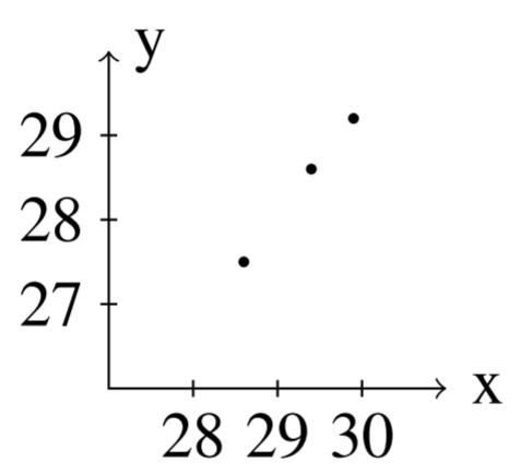
Then, we can find solutions for various values of $n$. Here are the solutions for values of $n$ between $1$ and $5$: $n=1: \left[ \begin{array}{r} 25.0 \\ 20.0 \end{array} \right],\; n=2: \left[ \begin{array}{r} 27.5 \\ 25.0 \end{array} \right],\; n=3: \left[ \begin{array}{r} 28.75 \\ 27.5 \end{array} \right],\; n=4: \left[ \begin{array}{r} 29.375 \\ 28.75 \end{array} \right],\; n=5: \left[ \begin{array}{r} 29.688 \\ 29.375 \end{array} \right]$
Notice that as $n$ increases, we approach the vector given by $\left[ \begin{array}{c} 2x\_{0}-y\_{0} \\ 2x\_{0}-y\_{0} \end{array} \right] = \left[ \begin{array}{r} 2\left(20\right)- 10 \\ 2\left( 20 \right)-10 \end{array} \right] = \left[ \begin{array}{r} 30 \\ 30 \end{array} \right] $
These solutions are graphed in the following figure.
The following example demonstrates another system which exhibits some interesting behavior. When we graph the solutions, it is possible for the ordered pairs to spiral around the origin.
Example 10: Finding Solutions to a Dynamical System 例 10:求动力系统的解
Suppose a dynamical system is of the form $\left[ \begin{array}{c} x\left( n+1\right) \\ y\left( n+1\right) \end{array} \right] =\left[ \begin{array}{rr} 0.7 & 0.7 \\ -0.7 & 0.7 \end{array} \right] \left[ \begin{array}{c} x\left( n\right) \\ y\left( n\right) \end{array} \right] $ Find solutions to the dynamical system for given initial conditions.
Solution 解
Let $A = \left[ \begin{array}{rr} 0.7 & 0.7 \\ -0.7 & 0.7 \end{array} \right] $ To find solutions, we must diagonalize $A$. You can verify that the eigenvalues of $A$ are complex and are given by $\lambda\_1 = .7+.7i$ and $\lambda\_2 = .7-.7i$. The eigenvector for $\lambda\_1 = .7+.7i$ is $\left[ \begin{array}{r} 1 \\ i \end{array} \right] $ and that the eigenvector for $\lambda\_2 = .7-.7i$ is $\left[ \begin{array}{r} 1 \\ -i \end{array} \right] $
Thus the matrix $A$ can be written in the form $\left[ \begin{array}{rr} 1 & 1 \\ i & -i \end{array} \right] \left[ \begin{array}{cc} .7+.7i & 0 \\ 0 & .7-.7i \end{array} \right] \left[ \begin{array}{rr} \frac{1}{2} & - \frac{1}{2}i \\ \frac{1}{2} & \frac{1}{2}i \end{array} \right] $ and so, $\begin{aligned} V\_n &= PD^nP^{-1}V\_0 \\ \left[ \begin{array}{c} x\left( n\right) \\ y\left( n\right) \end{array} \right] &=\left[ \begin{array}{rr} 1 & 1 \\ i & -i \end{array} \right] \left[ \begin{array}{cc} \left( .7+.7i\right) ^{n} & 0 \\ 0 & \left( .7-.7i\right) ^{n} \end{array} \right] \left[ \begin{array}{rr} \frac{1}{2} & - \frac{1}{2}i \\ \frac{1}{2} & \frac{1}{2}i \end{array} \right] \left[ \begin{array}{c} x\_{0} \\ y\_{0} \end{array} \right] \end{aligned}$
The explicit solution is given by $\left[ \begin{array}{c} x\_{0}\left( \frac{1}{2}\left( 0.7-0.7i \right) ^{n}+ \frac{1}{2} \left( 0.7+0.7i\right) ^{n}\right) + y\_{0}\left( \frac{1}{2} i\left( 0.7-0.7i\right) ^{n}-\frac{1}{2}i \left( 0.7+0.7i\right) ^{n}\right) \\ y\_{0}\left( \frac{1}{2} \left( 0.7-0.7i \right) ^{n}+ \frac{1}{2} \left( 0.7+0.7i\right) ^{n}\right) - x\_{0}\left( \frac{1}{2} i\left( 0.7-0.7i\right) ^{n}- \frac{1}{2}i\left( 0.7+0.7i\right) ^{n}\right) \end{array} \right] $
Suppose the initial condition is $\left[ \begin{array}{c} x\_{0} \\ y\_{0} \end{array} \right] =\left[ \begin{array}{r} 10 \\ 10 \end{array} \right] $ Then one obtains the following sequence of values which are graphed below by letting $n=1,2,\cdots ,20$
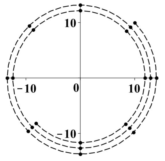
In this picture, the dots are the values and the dashed line is to help to picture what is happening.
These points are getting gradually closer to the origin, but they are circling the origin in the clockwise direction as they do so. As $n$ increases, the vector $\left[ \begin{array}{c} x\left( n\right) \\ y\left( n\right) \end{array} \right] $ approaches $\left[ \begin{array}{r} 0 \\ 0 \end{array} \right] $
This type of behavior along with complex eigenvalues is typical of the deviations from an equilibrium point in the Lotka Volterra system of differential equations which is a famous model for predator-prey interactions. These differential equations are given by $\begin{aligned} x^{\prime } &=x\left( a-by\right) \\ y^{\prime } &=-y\left( c-dx\right)\end{aligned}$ where $a,b,c,d$ are positive constants. For example, you might have $X$ be the population of moose and $Y$ the population of wolves on an island.
Note that these equations make logical sense. The top says that the rate at which the moose population increases would be $aX$ if there were no predators $Y$. However, this is modified by multiplying instead by $\left( a-bY\right)$ because if there are predators, these will militate against the population of moose. The more predators there are, the more pronounced is this effect. As to the predator equation, you can see that the equations predict that if there are many prey around, then the rate of growth of the predators would seem to be high. However, this is modified by the term $-cY$ because if there are many predators, there would be competition for the available food supply and this would tend to decrease $Y^{\prime }.$
The behavior near an equilibrium point, which is a point where the right side of the differential equations equals zero, is of great interest. In this case, the equilibrium point is $x=\frac{c}{d}, y=\frac{a}{b}$ Then one defines new variables according to the formula $x+\frac{c}{d}=x,\; y=y+\frac{a}{b}$ In terms of these new variables, the differential equations become $\begin{aligned} x^{\prime } &=\left( x+\frac{c}{d}\right) \left( a-b\left( y+\frac{a}{b} \right) \right) \\ y^{\prime } &=-\left( y+\frac{a}{b}\right) \left( c-d\left( x+\frac{c}{d} \right) \right)\end{aligned}$ Multiplying out the right sides yields $\begin{aligned} x^{\prime } &=-bxy-b\frac{c}{d}y \\ y^{\prime } &=dxy+\frac{a}{b}dx\end{aligned}$ The interest is for $x,y$ small and so these equations are essentially equal to $x^{\prime }=-b\frac{c}{d}y,\; y^{\prime }=\frac{a}{b}dx$
Replace $x^{\prime }$ with the difference quotient $\frac{x\left( t+h\right) -x\left( t\right) }{h}$ where $h$ is a small positive number and $y^{\prime }$ with a similar difference quotient. For example one could have $h$ correspond to one day or even one hour. Thus, for $h$ small enough, the following would seem to be a good approximation to the differential equations. $\begin{aligned} x\left( t+h\right) &=x\left( t\right) -hb\frac{c}{d}y \\ y\left( t+h\right) &=y\left( t\right) +h\frac{a}{b}dx\end{aligned}$ Let $1,2,3,\cdots$ denote the ends of discrete intervals of time having length $h$ chosen above. Then the above equations take the form $\left[ \begin{array}{c} x\left( n+1\right) \\ y\left( n+1\right) \end{array} \right] =\left[ \begin{array}{cc} 1 & - \frac{hbc}{d} \\ \frac{had}{b} & 1 \end{array} \right] \left[ \begin{array}{c} x\left( n\right) \\ y\left( n\right) \end{array} \right] $ Note that the eigenvalues of this matrix are always complex.
We are not interested in time intervals of length $h$ for $h$ very small. Instead, we are interested in much longer lengths of time. Thus, replacing the time interval with $mh,$ $\left[ \begin{array}{c} x\left( n+m\right) \\ y\left( n+m\right) \end{array} \right] =\left[ \begin{array}{cc} 1 & - \frac{hbc}{d} \\ \frac{had}{b} & 1 \end{array} \right] ^{m}\left[ \begin{array}{c} x\left( n\right) \\ y\left( n\right) \end{array} \right] $ For example, if $m=2,$ you would have $\left[ \begin{array}{c} x\left( n+2\right) \\ y\left( n+2\right) \end{array} \right] =\left[ \begin{array}{cc} 1-ach^{2} & -2b \frac{c}{d}h \\ 2 \frac{a}{b}dh & 1-ach^{2} \end{array} \right] \left[ \begin{array}{c} x\left( n\right) \\ y\left( n\right) \end{array} \right] $ Note that most of the time, the eigenvalues of the new matrix will be complex.
You can also notice that the upper right corner will be negative by considering higher powers of the matrix. Thus letting $1,2,3,\cdots$ denote the ends of discrete intervals of time, the desired discrete dynamical system is of the form $\left[ \begin{array}{c} x\left( n+1\right) \\ y\left( n+1\right) \end{array} \right] =\left[ \begin{array}{rr} a & -b \\ c & d \end{array} \right] \left[ \begin{array}{c} x\left( n\right) \\ y\left( n\right) \end{array} \right] $ where $a,b,c,d$ are positive constants and the matrix will likely have complex eigenvalues because it is a power of a matrix which has complex eigenvalues.
You can see from the above discussion that if the eigenvalues of the matrix used to define the dynamical system are less than 1 in absolute value, then the origin is stable in the sense that as $n\rightarrow \infty ,$ the solution converges to the origin. If either eigenvalue is larger than 1 in absolute value, then the solutions to the dynamical system will usually be unbounded, unless the initial condition is chosen very carefully. The next example exhibits the case where one eigenvalue is larger than 1 and the other is smaller than 1.
The following example demonstrates a familiar concept as a dynamical system.
Example 11: The Fibonacci Sequence 例 11:斐波那契数列
The Fibonacci sequence is the sequence given by $1, 1, 2, 3, 5, \cdots$ which is defined recursively in the form $x\left( 0\right) =1=x\left( 1\right) ,\; x\left( n+2\right) =x\left( n+1\right) +x\left( n\right)$ Show how the Fibonacci Sequence can be considered a dynamical system.
Solution 解
This sequence is extremely important in the study of reproducing rabbits. It can be considered as a dynamical system as follows. Let $y\left( n\right) =x\left( n+1\right) .$ Then the above recurrence relation can be written as $\left[ \begin{array}{c} x\left( n+1\right) \\ y\left( n+1\right) \end{array} \right] =\left[ \begin{array}{rr} 0 & 1 \\ 1 & 1 \end{array} \right] \left[ \begin{array}{c} x\left( n\right) \\ y\left( n\right) \end{array} \right] ,\; \left[ \begin{array}{c} x\left( 0\right) \\ y\left( 0\right) \end{array} \right] =\left[ \begin{array}{r} 1 \\ 1 \end{array} \right] $
Let $A = \left[ \begin{array}{rr} 0 & 1 \\ 1 & 1 \end{array} \right] $
The eigenvalues of the matrix $A$ are $\lambda\_1 = \frac{1}{2}-\frac{1}{2}\sqrt{5}$ and $\lambda\_2 = \frac{1}{2}\sqrt{5}+\frac{1}{2}$. The corresponding eigenvectors are, respectively, $X\_1 = \left[ \begin{array}{c} - \frac{1}{2}\sqrt{5}- \frac{1}{2} \\ 1 \end{array} \right] , X\_2 = \left[ \begin{array}{c} \frac{1}{2}\sqrt{5}- \frac{1}{2} \\ 1 \end{array} \right] $
You can see from a short computation that one of the eigenvalues is smaller than 1 in absolute value while the other is larger than 1 in absolute value. Now, diagonalizing $A$ gives us $\left[ \begin{array}{cc} \frac{1}{2}\sqrt{5}- \frac{1}{2} & - \frac{1}{2}\sqrt{5}- \frac{1}{2} \\ 1 & 1 \end{array} \right] ^{-1}\left[ \begin{array}{rr} 0 & 1 \\ 1 & 1 \end{array} \right] \left[ \begin{array}{cc} \frac{1}{2}\sqrt{5}- \frac{1}{2} & - \frac{1}{2}\sqrt{5}- \frac{1}{2} \\ 1 & 1 \end{array} \right] = \left[ \begin{array}{cc} \frac{1}{2}\sqrt{5}+ \frac{1}{2} & 0 \\ 0 & \frac{1}{2}- \frac{1}{2}\sqrt{5} \end{array} \right] $
Then it follows that for a given initial condition, the solution to this dynamical system is of the form $\begin{aligned} \left[ \begin{array}{c} x\left( n\right) \\ y\left( n\right) \end{array} \right] &=\left[ \begin{array}{cc} \frac{1}{2}\sqrt{5}- \frac{1}{2} & - \frac{1}{2}\sqrt{5}- \frac{1}{2} \\ 1 & 1 \end{array} \right] \left[ \begin{array}{cc} \left( \frac{1}{2}\sqrt{5}+ \frac{1}{2}\right) ^{n} & 0 \\ 0 & \left( \frac{1}{2}- \frac{1}{2}\sqrt{5}\right) ^{n} \end{array} \right] \cdot \left[ \begin{array}{cc} \frac{1}{5}\sqrt{5} & \frac{1}{10}\sqrt{5}+ \frac{1}{2} \\ - \frac{1}{5}\sqrt{5} & \frac{1}{5}\sqrt{5}\left( \frac{1}{2}\sqrt{5}- \frac{1}{2}\right) \end{array} \right] \left[ \begin{array}{r} 1 \\ 1 \end{array} \right] \end{aligned}$ It follows that $x\left( n\right) =\left( \frac{1}{2}\sqrt{5}+\frac{1}{2}\right) ^{n}\left( \frac{1}{10}\sqrt{5}+\frac{1}{2}\right) +\left( \frac{1}{2}-\frac{1}{2}\sqrt{5}\right) ^{n}\left( \frac{1}{2}-\frac{1}{10}\sqrt{5}\right) $
Here is a picture of the ordered pairs $\left( x\left( n\right) ,y\left( n\right) \right)$ for $n=0,1,\cdots ,n$.
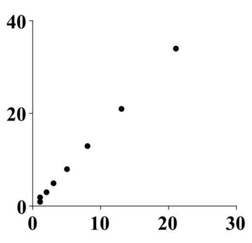
There is so much more that can be said about dynamical systems. It is a major topic of study in differential equations and what is given above is just an introduction.
The Matrix Exponential 矩阵指数
The goal of this section is to use the concept of the matrix exponential to solve first order linear differential equations. We begin by proving the matrix exponential.
Suppose $A$ is a diagonalizable matrix. Then the **matrix exponential**, written $e^{A}$, can be easily defined. Recall that if $D$ is a diagonal matrix, then $P^{-1}AP=D $ $D$ is of the form $\left $$ \begin{array}{ccc} \lambda \_{1} & & 0 \\ & \ddots & \\ 0 & & \lambda \_{n} \end{array} \right $$ \label{diagonalmatrix}$ and it follows that $D^{m}=\left $$ \begin{array}{ccc} \lambda \_{1}^{m} & & 0 \\ & \ddots & \\ 0 & & \lambda \_{n}^{m} \end{array} \right $$ $
Since $A$ is diagonalizable, $A=PDP^{-1} $ and $A^{m}=PD^{m}P^{-1} $
Recall why this is true. $A=PDP^{-1} $ and so $\begin{aligned} A^{m} &=\overset{ \text{m times}}{\overbrace{PDP^{-1}PDP^{-1}PDP^{-1}\cdots PDP^{-1}}} \\ &=PD^{m}P^{-1}\end{aligned}$$
We now will examine what is meant by the matrix exponental $e^{A}$. Begin by formally writing the following power series for $e^{A}$: $e^{A} = \sum\_{k=0}^{\infty }\frac{A^{k}}{k!}=\sum\_{k=0}^{\infty }\frac{PD^{k}P^{-1}}{k!}=P \left( \sum\_{k=0}^{\infty }\frac{D^{k}}{k!} \right)P^{-1} $ If $D$ is given above in $\eqref{diagonalmatrix}$, the above sum is of the form $P \left( \sum\_{k=0}^{\infty }\left $$ \begin{array}{ccc} \frac{1}{k!}\lambda \_{1}^{k} & & 0 \\ & \ddots & \\ 0 & & \frac{1}{k!}\lambda \_{n}^{k} \end{array} \right $$ \right) P^{-1} $ This can be rearranged as follows: $e^{A}=P\left $$ \begin{array}{ccc} \sum\_{k=0}^{\infty }\frac{1}{k!}\lambda \_{1}^{k} & & 0 \\ & \ddots & \\ 0 & & \sum\_{k=0}^{\infty }\frac{1}{k!}\lambda \_{n}^{k} \end{array} \right $$ P^{-1} $ $=P\left $$ \begin{array}{ccc} e^{\lambda \_{1}} & & 0 \\ & \ddots & \\ 0 & & e^{\lambda \_{n}} \end{array} \right $$ P^{-1} $
This justifies the following theorem.
Theorem 4: The Matrix Exponential 定理 4:矩阵指数
Let $A$ be a diagonalizable matrix, with eigenvalues $\lambda_1, ..., \lambda_n$and corresponding matrix of eigenvectors $P$. Then the matrix exponential, $e^{A}$, is given by $e^{A} = P\left $$ \begin{array}{ccc} e^{\lambda \_{1}} & & 0 \\ & \ddots & \\ 0 & & e^{\lambda \_{n}} \end{array} \right $$ P^{-1} $
Example 12: Compute $e^A$ for a Matrix $A$ 例 12:求矩阵 $A$ 的 $e^A$
Let $A=\left $$ \begin{array}{rrr} 2 & -1 & -1 \\ 1 & 2 & 1 \\ -1 & 1 & 2 \end{array} \right $$ $ Find $e^{A}$.
Solution 解
The eigenvalues work out to be $1,2,3$ and eigenvectors associated with these eigenvalues are $\left $$ \begin{array}{r} 0 \\ -1 \\ 1 \end{array} \right $$ \leftrightarrow 1, \left $$ \begin{array}{r} -1 \\ -1 \\ 1 \end{array} \right $$ \leftrightarrow 2,\left $$ \begin{array}{r} -1 \\ 0 \\ 1 \end{array} \right $$ \leftrightarrow 3 $ Then let $D=\left $$ \begin{array}{rrr} 1 & 0 & 0 \\ 0 & 2 & 0 \\ 0 & 0 & 3 \end{array} \right $$, P=\left $$ \begin{array}{rrr} 0 & -1 & -1 \\ -1 & -1 & 0 \\ 1 & 1 & 1 \end{array} \right $$ $ and so $P^{-1}=\left $$ \begin{array}{rrr} 1 & 0 & 1 \\ -1 & -1 & -1 \\ 0 & 1 & 1 \end{array} \right $$ $
Then the matrix exponential is $e^{At} = \left $$ \begin{array}{rrr} 0 & -1 & -1 \\ -1 & -1 & 0 \\ 1 & 1 & 1 \end{array} \right $$ \left $$ \begin{array}{ccc} e^{1} & 0 & 0 \\ 0 & e^{2} & 0 \\ 0 & 0 & e^{3} \end{array} \right $$ \left $$ \begin{array}{rrr} 1 & 0 & 1 \\ -1 & -1 & -1 \\ 0 & 1 & 1 \end{array} \right $$ $ $\left $$ \begin{array}{ccc} e^{2} & e^{2}-e^{3} & e^{2}-e^{3} \\ e^{2}-e & e^{2} & e^{2}-e \\ -e^{2}+e & -e^{2}+e^{3} & -e^{2}+e+e^{3} \end{array} \right $$ $
The matrix exponential is a useful tool to solve autonomous systems of first order linear differential equations. These are equations which are of the form $X^{\prime }=AX, X(0) = C $ where $A$ is a diagonalizable $n\times n$ matrix and $C$ is a constant vector. $X$ is a vector of functions in one variable, $t$: $X = X(t) = \left $$ \begin{array}{c} x_1(t) \\ x_2(t) \\ \vdots \\ x_n(t) \end{array} \right $$ $ Then $X^{\prime }$ refers to the first derivative of $X$ and is given by $X^{\prime} = X^{\prime}(t) = \left $$ \begin{array}{c} x_1^{\prime}(t) \\ x_2^{\prime}(t) \\ \vdots \\ x_n^{\prime}(t) \end{array} \right $$, $ x_i^{\prime}(t) = \text{the derivative of}$ x_i(t) $
Then it turns out that the solution to the above system of equations is $X\left( t\right) =e^{At}C$. To see this, suppose $A$ is diagonalizable so that $A=P\left $$ \begin{array}{ccc} \lambda \_{1} & & \\ & \ddots & \\ & & \lambda \_{n} \end{array} \right $$ P^{-1} $ Then $e^{At}=P\left $$ \begin{array}{ccc} e^{\lambda \_{1}t} & & \\ & \ddots & \\ & & e^{\lambda \_{n}t} \end{array} \right $$ P^{-1} $ $e^{At}C=P\left $$ \begin{array}{ccc} e^{\lambda \_{1}t} & & \\ & \ddots & \\ & & e^{\lambda \_{n}t} \end{array} \right $$ P^{-1}C $
Differentiating $e^{At}C$ yields $X^{\prime} = \left( e^{At}C\right) ^{\prime }=P\left $$ \begin{array}{ccc} \lambda \_{1}e^{\lambda \_{1}t} & & \\ & \ddots & \\ & & \lambda \_{n}e^{\lambda \_{n}t} \end{array} \right $$ P^{-1}C $ $=P\left $$ \begin{array}{ccc} \lambda \_{1} & & \\ & \ddots & \\ & & \lambda \_{n} \end{array} \right $$ \left $$ \begin{array}{ccc} e^{\lambda \_{1}t} & & \\ & \ddots & \\ & & e^{\lambda \_{n}t} \end{array} \right $$ P^{-1}C $ $\begin{aligned} &=P\left && \begin{array}{ccc} \lambda \_{1} & & \\ & \ddots & \\ & & \lambda \_{n} \end{array} \right $$ P^{-1}P\left $$ \begin{array}{ccc} e^{\lambda \_{1}t} & & \\ & \ddots & \\ & & e^{\lambda \_{n}t} \end{array} \right $$ P^{-1}C $ &=A\left( e^{At}C\right) = AX\end{aligned}$ Therefore $X = X(t) = e^{At}C$ is a solution to $X^{\prime }=AX$.$
To prove that $X(0) = C$ if $X(t) = e^{At}C$: $X(0) = e^{A0}C=P\left $$ \begin{array}{ccc} 1 & & \\ & \ddots & \\ & & 1 \end{array} \right $$ P^{-1}C=C $
Example 13: Solving an Initial Value Problem 例 13:求解初值问题
Solve the initial value problem $\left $$ \begin{array}{c} x \\ y \end{array} \right $$ ^{\prime }=\left $$ \begin{array}{rr} 0 & -2 \\ 1 & 3 \end{array} \right $$ \left $$ \begin{array}{c} x \\ y \end{array} \right $$ ,$ \left $$ \begin{array}{c} x(0)& y(0) \end{array} \right $$ =\left $$ \begin{array}{c} 1 \\ 1 \end{array} \right $$ $
Solution 解
The matrix is diagonalizable and can be written as $\begin{aligned} A &= PDP^{-1} \\ \left && \begin{array}{rr} 0 & -2 \\ 1 & 3 \end{array} \right $$ &=\left $$ \begin{array}{rr} 1 & 1 \\ -\frac{1}{2} & -1 \end{array} \right $$ \left $$ \begin{array}{rr} 1 & 0 \\ 0 & 2 \end{array} \right $$ \left $$ \begin{array}{rr} 2 & 2 \\ -1 & -2 \end{array} \right $$\end{aligned}$ Therefore, the matrix exponential is of the form $e^{At} = \left $$ \begin{array}{rr} 1 & 1 \\ -\frac{1}{2} & -1 \end{array} \right $$ \left $$ \begin{array}{cc} e^{t} & 0 \\ 0 & e^{2t} \end{array} \right $$ \left $$ \begin{array}{rr} 2 & 2 \\ -1 & -2 \end{array} \right $$ $ The solution to the initial value problem is $\begin{aligned} X(t) &= e^{At}C \\ \left && \begin{array}{c} x\left( t\right) \\ y\left( t\right) \end{array} \right $$ &= \left $$ \begin{array}{rr} 1 & 1 \\ -\frac{1}{2} & -1 \end{array} \right $$ \left $$ \begin{array}{cc} e^{t} & 0 \\ 0 & e^{2t} \end{array} \right $$ \left $$ \begin{array}{rr} 2 & 2 \\ -1 & -2 \end{array} \right $$ \left $$ \begin{array}{c} 1 \\ 1 \end{array} \right $$ $ &=\left $$ \begin{array}{c} 4e^{t}-3e^{2t} \\ 3e^{2t}-2e^{t} \end{array} \right $$\end{aligned}$ We can check that this works: $\begin{aligned} \left && \begin{array}{c} x\left( 0\right) \\ y\left( 0\right) \end{array} \right $$ &= \left $$ \begin{array}{c} 4e^{0}-3e^{2(0)} \\ 3e^{2(0)}-2e^{0} \end{array} \right $$ $ &= \left $$ \begin{array}{c} 1 \\ 1 \end{array} \right $$\end{aligned}$
Lastly, $X^{\prime} = \left $$ \begin{array}{c} 4e^{t}-3e^{2t} \\ 3e^{2t}-2e^{t} \end{array} \right $$ ^{\prime }=\left $$ \begin{array}{c} 4e^{t}-6e^{2t} \\ 6e^{2t}-2e^{t} \end{array} \right $$ $ and $AX = \left $$ \begin{array}{rr} 0 & -2 \\ 1 & 3 \end{array} \right $$ \left $$ \begin{array}{c} 4e^{t}-3e^{2t} \\ 3e^{2t}-2e^{t} \end{array} \right $$ =\left $$ \begin{array}{c} 4e^{t}-6e^{2t} \\ 6e^{2t}-2e^{t} \end{array} \right $$ $ which is the same thing. Thus this is the solution to the initial value problem.$
Orthogonal Diagonalization 正交对角化
We begin this section by recalling some important definitions. Recall from Definition 4.11.4 that non-zero vectors are called orthogonal if their dot product equals $0$. A set is orthonormal if it is orthogonal and each vector is a unit vector.
An orthogonal matrix $U$, from Definition 4.11.7, is one in which $UU^{T} = I$. In other words, the transpose of an orthogonal matrix is equal to its inverse. A key characteristic of orthogonal matrices, which will be essential in this section, is that the columns of an orthogonal matrix form an orthonormal set.
We now recall another important definition.
Definition 1: Symmetric and Skew Symmetric Matrices 定义 1:对称矩阵与反对称矩阵
A real $n\times n$ matrix $A,$ is **symmetric** if $A^{T}=A.$ If $ A=-A^{T},$ then $A$ is called **skew symmetric.**
Before proving an essential theorem, we first examine the following lemma which will be used below.
Lemma 1: The Dot Product 引理 1:点积
Let $A=\left ( a\_{ij} \right )$ be a real symmetric $n \times n$ matrix, and let $\vec{x}, \vec{y} \in \mathbb{R}^n$. Then $A\vec{x} \cdot \vec{y} = \vec{x} \cdot A \vec{y}$
Proof. This result follows from the definition of the dot product together with properties of matrix multiplication, as follows: $\begin{aligned} A\vec{x} \cdot \vec{y} &= \sum\_{k,l}a\_{kl}x\_{l}y\_{k} \\ &=\sum\_{k,l} (a\_{lk})^Tx\_{l}y\_{k} \\ &= \vec{x}\cdot A^{T}\vec{y} \\ &= \vec{x}\cdot A \vec{y}\end{aligned}$$
The last step follows from $A^T = A$, since $A$ is symmetric.
We can now prove that the eigenvalues of a real symmetric matrix are real numbers. Consider the following important theorem.
Theorem 1: Orthogonal Eigenvectors 定理 1:正交的特征向量
Let $A$ be a real symmetric matrix. Then the eigenvalues of $A$ are real numbers and eigenvectors corresponding to distinct eigenvalues are orthogonal.
Proof. Recall that for a complex number $a+ib,$ the complex conjugate, denoted by $\overline{a+ib}$ is given by $\overline{a+ib}=a-ib.$ The notation, $\overline{\vec{x}}$ will denote the vector which has every entry replaced by its complex conjugate.
Suppose $A$ is a real symmetric matrix and $A\vec{x}=\lambda \vec{x}$. Then $\overline{\lambda \vec{x}}^{T}\vec{x}=\left( \overline{A \vec{x}}\right) ^{T}\vec{x}=\overline{\vec{x}}^{T}A^{T}\vec{x}= \overline{\vec{x}}^{T}A\vec{x}=\lambda \overline{\vec{x}}^{T} \vec{x} $ Dividing by $\overline{\vec{x}}^{T}\vec{x}$ on both sides yields $\overline{\lambda }=\lambda$ which says $\lambda$ is real. To do this, we need to ensure that $\overline{\vec{x}}^{T}\vec{x} \neq 0$. Notice that $\overline{\vec{x}}^{T}\vec{x} = 0$ if and only if $\vec{x} = \vec{0}$. Since we chose $\vec{x}$ such that $A\vec{x} = \lambda \vec{x}$, $\vec{x}$ is an eigenvector and therefore must be nonzero.
Now suppose $A$ is real symmetric and $A\vec{x}=\lambda \vec{x}$, $A \vec{y}=\mu \vec{y}$ where $\mu \neq \lambda$. Then since $A$ is symmetric, it follows from Lemma $\PageIndex{1}$ about the dot product that $\lambda \vec{x}\cdot \vec{y}=A\vec{x}\cdot \vec{y}=\vec{x}\cdot A\vec{y}=\vec{x}\cdot \mu \vec{y}=\mu \vec{x}\cdot \vec{y} $ Hence $\left( \lambda -\mu \right) \vec{x}\cdot \vec{y}=0.$ It follows that, since $\lambda -\mu \neq 0,$ it must be that $\vec{x}\cdot \vec{y}=0$. Therefore the eigenvectors form an orthogonal set.
The following theorem is proved in a similar manner.
Theorem 2: Eigenvalues of Skew Symmetric Matrix 定理 2:反对称矩阵的特征值
The eigenvalues of a real skew symmetric matrix are either equal to $0$ or are pure imaginary numbers.
Proof. First, note that if $A=0$ is the zero matrix, then $A$ is skew symmetric and has eigenvalues equal to $0$.
Suppose $A=-A^{T}$ so $A$ is skew symmetric and $A\vec{x}=\lambda \vec{x}$. Then $\overline{\lambda \vec{x}}^{T}\vec{x}=\left( \overline{A \vec{x}}\right) ^{T}\vec{x}=\overline{\vec{x}}^{T}A^{T}\vec{x}=- \overline{\vec{x}}^{T}A\vec{x}=-\lambda \overline{\vec{x}}^{T} \vec{x} $ and so, dividing by $\overline{\vec{x}}^{T}\vec{x}$ as before, $\overline{\lambda }=-\lambda .$ Letting $\lambda =a+ib,$ this means $a-ib=-a-ib$ and so $a=0.$ Thus $\lambda$ is pure imaginary.
Consider the following example.
Example 1: Eigenvalues of a Skew Symmetric Matrix 例 1:反对称矩阵的特征值
Let $A=\left[ \begin{array}{rr} 0 & -1 \\ 1 & 0 \end{array} \right] .$ Find its eigenvalues.$
Solution 解
First notice that $A$ is skew symmetric. By Theorem $\PageIndex{2}$, the eigenvalues will either equal $0$ or be pure imaginary. The eigenvalues of $A$ are obtained by solving the usual equation $\det (\lambda I - A ) = \det \left[ \begin{array}{rr} \lambda & 1 \\ -1 & \lambda \end{array} \right] =\lambda ^{2}+1=0 $$
Hence the eigenvalues are $\pm i,$ pure imaginary.
Consider the following example.
Example 2: Eigenvalues of a Symmetric Matrix 例 2:对称矩阵的特征值
Let $A=\left[ \begin{array}{rr} 1 & 2 \\ 2 & 3 \end{array} \right] .$ Find its eigenvalues.$
Solution 解
First, notice that $A$ is symmetric. By Theorem $\PageIndex{1}$, the eigenvalues will all be real. The eigenvalues of $A$ are obtained by solving the usual equation $\det (\lambda I - A) = \det \left[ \begin{array}{rr} \lambda - 1 & -2 \\ -2 & \lambda - 3 \end{array} \right] = \lambda^2 -4\lambda -1=0 $ The eigenvalues are given by $\lambda_1 =2+ \sqrt{5}$ and $\lambda_2 =2-\sqrt{5}$ which are both real.$
Recall that a diagonal matrix $D=\left ( d\_{ij} \right )$ is one in which $d\_{ij} = 0$ whenever $i \neq j$. In other words, all numbers not on the main diagonal are equal to zero.
Consider the following important theorem.
Theorem 3: Orthogonal Diagonalization 定理 3:正交对角化
Let $A$ be a real symmetric matrix. Then there exists an orthogonal matrix $U$ such that $U^{T}AU = D $ where $D$ is a diagonal matrix. Moreover, the diagonal entries of $D$ are the eigenvalues of $A$.
We can use this theorem to diagonalize a symmetric matrix, using orthogonal matrices. Consider the following corollary.
Corollary 1: Orthonormal Set of Eigenvectors 推论 1:特征向量的标准正交组
If $A$ is a real $n\times n$ symmetric matrix, then there exists an orthonormal set of eigenvectors, $\left\{ \vec{u}\_{1},\cdots ,\vec{u} \_{n}\right\} .$
Proof. Since $A$ is symmetric, then by Theorem $\PageIndex{3}$, there exists an orthogonal matrix $U$ such that $U^{T}AU=D,$ a diagonal matrix whose diagonal entries are the eigenvalues of $A.$ Therefore, since $A$ is symmetric and all the matrices are real, $\overline{D}=\overline{D^{T}}=\overline{U^{T}A^{T}U}=U^{T}A^{T}U=U^{T}AU=D $ showing $D$ is real because each entry of $D$ equals its complex conjugate.
Now let $U=\left[ \begin{array}{cccc} \vec{u}\_{1} & \vec{u}\_{2} & \cdots & \vec{u}\_{n} \end{array} \right] $ where the $\vec{u}\_{i}$ denote the columns of $U$ and $D=\left[ \begin{array}{ccc} \lambda \_{1} & & 0 \\ & \ddots & \\ 0 & & \lambda \_{n} \end{array} \right] $ The equation, $U^{T}AU=D$ implies $AU = UD$ and $\begin{aligned} AU &=\left[ \begin{array}{cccc} A\vec{u}\_{1} & A\vec{u}\_{2} & \cdots & A\vec{u}\_{n} \end{array} \right] $ &=\left[ \begin{array}{cccc} \lambda \_{1}\vec{u}\_{1} & \lambda \_{2}\vec{u}\_{2} & \cdots & \lambda \_{n}\vec{u}\_{n} \end{array} \right] $ &= UD\end{aligned}$ where the entries denote the columns of $AU$ and $UD$ respectively. Therefore, $A\vec{u}\_{i}=\lambda \_{i}\vec{u}\_{i}$. Since the matrix $U$ is orthogonal, the $ij^{th}$ entry of $U^{T}U$ equals $\delta \_{ij}$ and so $\delta \_{ij}=\vec{u}\_{i}^{T}\vec{u}\_{j}=\vec{u}\_{i}\cdot \vec{u} \_{j} $ This proves the corollary because it shows the vectors $\left\{ \vec{u} \_{i}\right\} form an orthonormal set.$
Definition 2: Principal Axes 定义 2:主轴
Let $A$ be an $n \times n$ matrix. Then the principal axes of $A$ is a set of orthonormal eigenvectors of $A$.
In the next example, we examine how to find such a set of orthonormal eigenvectors.
Example 3: Find an Orthonormal Set of Eigenvectors 例 3:求一组标准正交特征向量
Find an orthonormal set of eigenvectors for the symmetric matrix $A = \left[ \begin{array}{rrr} 17 & -2 & -2 \\ -2 & 6 & 4 \\ -2 & 4 & 6 \end{array} \right] $
Solution 解
Recall Procedure 7.1.1 for finding the eigenvalues and eigenvectors of a matrix. You can verify that the eigenvalues are $18,9,2.$ First find the eigenvector for $18$ by solving the equation \$18I-A)X = 0$. The appropriate augmented matrix is given by $\left[ \begin{array}{ccc\|c} 18-17 & 2 & 2 & 0 \\ 2 & 18-6 & -4 & 0 \\ 2 & -4 & 18-6 & 0 \end{array} \right] $ The reduced row-echelon form is $\left[ \begin{array}{rrr\|r} 1 & 0 & 4 & 0 \\ 0 & 1 & -1 & 0 \\ 0 & 0 & 0 & 0 \end{array} \right] $ Therefore an eigenvector is $\left[ \begin{array}{r} -4 \\ 1 \\ 1 \end{array} \right] $ Next find the eigenvector for $\lambda =9.$ The augmented matrix and resulting reduced row-echelon form are $\left[ \begin{array}{ccc\|c} 9-17 & 2 & 2 & 0 \\ 2 & 9-6 & -4 & 0 \\ 2 & -4 & 9-6 & 0 \end{array} \right] \rightarrow \cdots \rightarrow \left[ \begin{array}{rrr\|r} 1 & 0 & - \frac{1}{2} & 0 \\ 0 & 1 & -1 & 0 \\ 0 & 0 & 0 & 0 \end{array} \right] $ Thus an eigenvector for $\lambda =9$ is $\left[ \begin{array}{r} 1 \\ 2 \\ 2 \end{array} \right] $ Finally find an eigenvector for $\lambda =2.$ The appropriate augmented matrix and reduced row-echelon form are $\left[ \begin{array}{ccc\|c} 2-17 & 2 & 2 & 0 \\ 2 & 2-6 & -4 & 0 \\ 2 & -4 & 2-6 & 0 \end{array} \right] \rightarrow \cdots \rightarrow \left[ \begin{array}{rrr\|r} 1 & 0 & 0 & 0 \\ 0 & 1 & 1 & 0 \\ 0 & 0 & 0 & 0 \end{array} \right] $ Thus an eigenvector for $\lambda =2$ is $\left[ \begin{array}{r} 0 \\ -1 \\ 1 \end{array} \right] $$
The set of eigenvectors for $A$ is given by $\left\{ \left[ \begin{array}{r} -4 \\ 1 \\ 1 \end{array} \right], \left[ \begin{array}{r} 1 \\ 2 \\ 2 \end{array} \right], \left[ \begin{array}{r} 0 \\ -1 \\ 1 \end{array} \right] \right\}nonumber $ You can verify that these eigenvectors form an orthogonal set. By dividing each eigenvector by its magnitude, we obtain an orthonormal set: $\left\{ \frac{1}{\sqrt{18}}\left[ \begin{array}{r} -4 \\ 1 \\ 1 \end{array} \right] ,\frac{1}{3}\left[ \begin{array}{r} 1 \\ 2 \\ 2 \end{array} \right] ,\frac{1}{\sqrt{2}}\left[ \begin{array}{r} 0 \\ -1 \\ 1 \end{array} \right] \right\}nonumber $
Consider the following example.
Example 4: Repeated Eigenvalues 例 4:重特征值
Find an orthonormal set of three eigenvectors for the matrix $A = \left[ \begin{array}{rrr} 10 & 2 & 2 \\ 2 & 13 & 4 \\ 2 & 4 & 13 \end{array} \right] $
Solution 解
You can verify that the eigenvalues of $A$ are $9$ (with multiplicity two) and $18$ (with multiplicity one). Consider the eigenvectors corresponding to $\lambda =9$. The appropriate augmented matrix and reduced row-echelon form are given by $\left[ \begin{array}{ccc\|c} 9-10 & -2 & -2 & 0 \\ -2 & 9-13 & -4 & 0 \\ -2 & -4 & 9-13 & 0 \end{array} \right] \rightarrow \cdots \rightarrow \left[ \begin{array}{rrr\|r} 1 & 2 & 2 & 0 \\ 0 & 0 & 0 & 0 \\ 0 & 0 & 0 & 0 \end{array} \right] $ and so eigenvectors are of the form $\left[ \begin{array}{c} -2y-2z \\ y \\ z \end{array} \right] $ We need to find two of these which are orthogonal. Let one be given by setting $z=0$ and $y=1$, giving $\left[ \begin{array}{r} -2 \\ 1 \\ 0 \end{array} \right]$.
In order to find an eigenvector orthogonal to this one, we need to satisfy $\left[ \begin{array}{r} -2 \\ 1 \\ 0 \end{array} \right] \cdot \left[ \begin{array}{c} -2y-2z \\ y \\ z \end{array} \right] =5y+4z=0 $ The values $y=-4$ and $z=5$ satisfy this equation, giving another eigenvector corresponding to $\lambda=9$ as $\left[ \begin{array}{c} -2\left( -4\right) -2\left( 5\right) \\ \left( -4\right) \\ 5 \end{array} \right] =\left[ \begin{array}{r} -2 \\ -4 \\ 5 \end{array} \right] $ Next find the eigenvector for $\lambda =18.$ The augmented matrix and the resulting reduced row-echelon form are given by $\left[ \begin{array}{ccc\|c} 18-10 & -2 & -2 & 0 \\ -2 & 18-13 & -4 & 0 \\ -2 & -4 & 18-13 & 0 \end{array} \right] \rightarrow \cdots \rightarrow \left[ \begin{array}{rrr\|r} 1 & 0 & - \frac{1}{2} & 0 \\ 0 & 1 & -1 & 0 \\ 0 & 0 & 0 & 0 \end{array} \right] $ and so an eigenvector is $\left[ \begin{array}{r} 1 \\ 2 \\ 2 \end{array} \right] $
Dividing each eigenvector by its length, the orthonormal set is $\left\{ \frac{1}{\sqrt{5}} \left[ \begin{array}{r} -2& 1 \\ 0 \end{array} \right] , \frac{\sqrt{5}}{15} \left[ \begin{array}{r} -2 \\ -4 \\ 5 \end{array} \right] , \frac{1}{3}\left[ \begin{array}{r} 1 \\ 2 \\ 2 \end{array} \right] \right\}nonumber $
In the above solution, the repeated eigenvalue implies that there would have been many other orthonormal bases which could have been obtained. While we chose to take $z=0, y=1$, we could just as easily have taken $y=0$ or even $y=z=1.$ Any such change would have resulted in a different orthonormal set.
Recall the following definition.
Definition 3: Diagonalizable 定义 3:可对角化
An $n\times n$ matrix $A$ is said to be **non defective** or **diagonalizable** if there exists an invertible matrix $P$ such that $P^{-1}AP=D$ where $D$ is a diagonal matrix.
As indicated in Theorem $\PageIndex{3}$ if $A$ is a real symmetric matrix, there exists an orthogonal matrix $U$ such that $U^{T}AU=D$ where $D$ is a diagonal matrix. Therefore, every symmetric matrix is diagonalizable because if $U$ is an orthogonal matrix, it is invertible and its inverse is $U^{T}$. In this case, we say that $A$ is **orthogonally diagonalizable**. Therefore every symmetric matrix is in fact orthogonally diagonalizable. The next theorem provides another way to determine if a matrix is orthogonally diagonalizable.
Theorem 4: Orthogonally Diagonalizable 定理 4:正交可对角化
Let $A$ be an $n \times n$ matrix. Then $A$ is orthogonally diagonalizable if and only if $A$ has an orthonormal set of eigenvectors.
Recall from Corollary $\PageIndex{1}$ that every symmetric matrix has an orthonormal set of eigenvectors. In fact these three conditions are equivalent.
In the following example, the orthogonal matrix $U$ will be found to orthogonally diagonalize a matrix.
Example 5: Diagonalize a Symmetric Matrix 例 5:对角化一个对称矩阵
Let $A=\left[ \begin{array}{rrr} 1 & 0 & 0 \\ 0 & \frac{3}{2} & \frac{1}{2} \\ 0 & \frac{1}{2} & \frac{3}{2} \end{array} \right] .$ Find an orthogonal matrix $U$ such that $U^{T}AU$ is a diagonal matrix.
Solution 解
In this case, the eigenvalues are $2$ (with multiplicity one) and $1$ (with multiplicity two). First we will find an eigenvector for the eigenvalue $2$. The appropriate augmented matrix and resulting reduced row-echelon form are given by $\left[ \begin{array}{ccc\|c} 2-1 & 0 & 0 & 0 \\ 0 & 2- \frac{3}{2} & - \frac{1}{2} & 0 \\ 0 & - \frac{1}{2} & 2- \frac{3}{2} & 0 \end{array} \right] \rightarrow \cdots \rightarrow \left[ \begin{array}{rrr\|r} 1 & 0 & 0 & 0 \\ 0 & 1 & -1 & 0 \\ 0 & 0 & 0 & 0 \end{array} \right] $ and so an eigenvector is $\left[ \begin{array}{r} 0 \\ 1 \\ 1 \end{array} \right] $ However, it is desired that the eigenvectors be unit vectors and so dividing this vector by its length gives $\left[ \begin{array}{c} 0 \\ \frac{1}{\sqrt{2}} \\ \frac{1}{\sqrt{2}} \end{array} \right] $ Next find the eigenvectors corresponding to the eigenvalue equal to $1$. The appropriate augmented matrix and resulting reduced row-echelon form are given by: $\left[ \begin{array}{ccc\|c} 1-1 & 0 & 0 & 0 \\ 0 & 1- \frac{3}{2} & - \frac{1}{2} & 0 \\ 0 & - \frac{1}{2} & 1- \frac{3}{2} & 0 \end{array} \right] \rightarrow \cdots \rightarrow \left[ \begin{array}{rrr\|r} 0 & 1 & 1 & 0 \\ 0 & 0 & 0 & 0 \\ 0 & 0 & 0 & 0 \end{array} \right] $ Therefore, the eigenvectors are of the form $\left[ \begin{array}{r} s \\ -t \\ t \end{array} \right] $ Two of these which are orthonormal are $\left[ \begin{array}{c} 1 \\ 0 \\ 0 \end{array} \right]$, choosing $s=1$ and $t=0$, and $\left[ \begin{array}{c} 0 \\ - \frac{1}{\sqrt{2}} \\ \frac{1}{\sqrt{2}} \end{array} \right]$, letting $s=0$, $t= 1$ and normalizing the resulting vector.
To obtain the desired orthogonal matrix, we let the orthonormal eigenvectors computed above be the columns. $\left[ \begin{array}{rrr} 0 & 1 & 0 \\ -\frac{1}{\sqrt{2}} & 0 & \frac{1}{\sqrt{2}} \\ \frac{1}{\sqrt{2}} & 0 & \frac{1}{\sqrt{2}} \end{array} \right] $
To verify, compute $U^{T}AU$ as follows: $U^{T}AU = \left[ \begin{array}{rrr} 0 & - \frac{1}{\sqrt{2}} & \frac{1}{\sqrt{2}} \\ 1 & 0 & 0 \\ 0 & \frac{1}{\sqrt{2}} & \frac{1}{\sqrt{2}} \end{array} \right] \left[ \begin{array}{rrr} 1 & 0 & 0 \\ 0 & \frac{3}{2} & \frac{1}{2} \\ 0 & \frac{1}{2} & \frac{3}{2} \end{array} \right] \left[ \begin{array}{rrr} 0 & 1 & 0 \\ -\frac{1}{\sqrt{2}} & 0 & \frac{1}{\sqrt{2}} \\ \frac{1}{\sqrt{2}} & 0 & \frac{1}{\sqrt{2}} \end{array} \right] $ $=\left[ \begin{array}{rrr} 1 & 0 & 0 \\ 0 & 1 & 0 \\ 0 & 0 & 2 \end{array} \right] = D $ the desired diagonal matrix. Notice that the eigenvectors, which construct the columns of $U$, are in the same order as the eigenvalues in $D$.
We conclude this section with a Theorem that generalizes earlier results.
Theorem 5: Triangulation of a Matrix 定理 5:矩阵三角化
Let $A$ be an $n \times n$ matrix. If $A$ has $n$ real eigenvalues, then an orthogonal matrix $U$ can be found to result in the upper triangular matrix $U^T A U$.
triangulation
This Theorem provides a useful Corollary.
Corollary 2: Determinant and Trace 推论 2:行列式与迹
Let $A$ be an $n \times n$ matrix with eigenvalues $\lambda_1, \cdots, \lambda_n$. Then it follows that $\det(A)$ is equal to the product of the $\lambda_i$, while $trace(A)$ is equal to the sum of the $\lambda_i$.
Proof. By Theorem $\PageIndex{5}$, there exists an orthogonal matrix $U$ such that $U^TAU=P$, where $P$ is an upper triangular matrix. Since $P$ is similar to $A$, the eigenvalues of $P$ are $\lambda_1, \lambda_2, \ldots, \lambda_n$. Furthermore, since $P$ is (upper) triangular, the entries on the main diagonal of $P$ are its eigenvalues, so $\det(P)=\lambda_1 \lambda_2 \cdots \lambda_n$ and $trace(P)=\lambda_1 + \lambda_2 + \cdots + \lambda_n$. Since $P$ and $A$ are similar, $\det(A)=\det(P)$ and $trace(A)=trace(P)$, and therefore the results follow.
The Singular Value Decomposition 奇异值分解
We begin this section with an important definition.
Definition 4: Singular Values 定义 4:奇异值
Let $A$ be an $m\times n$ matrix. The singular values of $A$ are the square roots of the positive eigenvalues of $A^TA.$
Singular Value Decomposition (SVD) can be thought of as a generalization of orthogonal diagonalization of a symmetric matrix to an arbitrary $m\times n$ matrix. This decomposition is the focus of this section.
The following is a useful result that will help when computing the SVD of matrices.
Proposition 1: Same Nonzero Eigenvalues 命题 1:相同的非零特征值
Let $A$ be an $m \times n$ matrix. Then $A^TA$ and $AA^T$ have the same nonzero eigenvalues.
Proof Suppose $A$ is an $m\times n$ matrix, and suppose that $\lambda$ is a nonzero eigenvalue of $A^TA$. Then there exists a nonzero vector $X\in \mathbb{R}^n$ such that (上式) $(A^TA)X=\lambda X.$
Multiplying both sides of this equation by $A$ yields: $\begin{aligned} A(A^TA)X & = A\lambda X& (AA^T)(AX) & = \lambda (AX).\end{aligned}$ Since $\lambda\neq 0$ and $X\neq 0_n$, $\lambda X\neq 0_n$, and thus by 上式, \$A^TA)X\neq 0_m$; thus $A^T(AX)\neq 0_m$, implying that $AX\neq 0_m$.
Therefore $AX$ is an eigenvector of $AA^T$ corresponding to eigenvalue $\lambda$. An analogous argument can be used to show that every nonzero eigenvalue of $AA^T$ is an eigenvalue of $A^TA$, thus completing the proof.
Given an $m\times n$ matrix $A$, we will see how to express $A$ as a product $A=U\Sigma V^T $ where
- $U$ is an $m\times m$ orthogonal matrix whose columns are eigenvectors of $AA^T$.
- $V$ is an $n\times n$ orthogonal matrix whose columns are eigenvectors of $A^TA$.
- $\Sigma$ is an $m\times n$ matrix whose only nonzero values lie on its main diagonal, and are the singular values of $A$.
- $U$ 是一个 $m\times m$ 正交矩阵,其列向量是 $AA^T$ 的特征向量。
- $V$ 是一个 $n\times n$ 正交矩阵,其列向量是 $A^TA$ 的特征向量。
- $\Sigma$ 是一个 $m\times n$ 矩阵,其唯一的非零元素位于主对角线上,且正好是 $A$ 的奇异值。
How can we find such a decomposition? We are aiming to decompose $A$ in the following form:
$$A=U\left[ \begin{array}{cc} \sigma & 0 \\ 0 & 0 \end{array} \right] V^T \\ where \\\sigma\\ is of the form \\\sigma =\left[ \begin{array}{ccc} \sigma \_{1} & & 0 \\ & \ddots & \\ 0 & & \sigma \_{k} \end{array} \right]$$
Thus $A^T=V\left[ \begin{array}{cc} \sigma & 0 \\ 0 & 0 \end{array} \right] U^T$ and it follows that $A^TA=V\left[ \begin{array}{cc} \sigma & 0 \\ 0 & 0 \end{array} \right] U^TU\left[ \begin{array}{cc} \sigma & 0 \\ 0 & 0 \end{array} \right] V^T=V\left[ \begin{array}{cc} \sigma ^{2} & 0 \\ 0 & 0 \end{array} \right] V^T $ and so $A^TAV=V\left[ \begin{array}{cc} \sigma ^{2} & 0 \\ 0 & 0 \end{array} \right] .$ Similarly, $AA^TU=U\left[ \begin{array}{cc} \sigma ^{2} & 0 \\ 0 & 0 \end{array} \right] .$ Therefore, you would find an orthonormal basis of eigenvectors for $AA^T$ make them the columns of a matrix such that the corresponding eigenvalues are decreasing. This gives $U.$ You could then do the same for $A^TA$ to get $V$.
We formalize this discussion in the following theorem.
Theorem 6: Singular Value Decomposition 定理 6:奇异值分解
Let $A$ be an $m\times n$ matrix. Then there exist orthogonal matrices $U$ and $V$ of the appropriate size such that $A= U \Sigma V^T$ where $\Sigma$ is of the form $\Sigma = \left[ \begin{array}{cc} \sigma & 0 \\ 0 & 0 \end{array} \right] $ and $\sigma$ is of the form $\sigma =\left[ \begin{array}{ccc} \sigma \_{1} & & 0 \\ & \ddots & \\ 0 & & \sigma \_{k} \end{array} \right] $ for the $\sigma \_{i}$ the singular values of $A.$$
Proof There exists an orthonormal basis, $\left\{ \vec{v}\_{i}\right\} \_{i=1}^{n}$ such that $A^TA\vec{v}\_{i}=\sigma \_{i}^{2}\vec{v}\_{i}$ where $\sigma \_{i}^{2}>0$ for $i=1,\cdots ,k,\left( \sigma \_{i}>0\right)$ and equals zero if $i>k.$ Thus for $i>k,$ $A\vec{v}\_{i}=\vec{0}$ because $A\vec{v}\_{i}\cdot A\vec{v}\_{i} = A^TA\vec{v}\_{i} \cdot \vec{v}\_{i} = \vec{0} \cdot \vec{v}\_{i} =0. $ For $i=1,\cdots ,k,$ define $\vec{u}\_{i}\in \mathbb{R}^{m}$ by $\vec{u}\_{i}= \sigma \_{i}^{-1}A\vec{v}\_{i}. $ Thus $A\vec{v}\_{i}=\sigma \_{i}\vec{u}\_{i}.$ Now $\begin{aligned} \vec{u}\_{i} \cdot \vec{u}\_{j} &= \sigma \_{i}^{-1}A \vec{v}\_{i} \cdot \sigma \_{j}^{-1}A\vec{v}\_{j} = \sigma\_{i}^{-1}\vec{v}\_{i} \cdot \sigma \_{j}^{-1}A^TA\vec{v}\_{j} \\ &= \sigma \_{i}^{-1}\vec{v}\_{i} \cdot \sigma \_{j}^{-1}\sigma \_{j}^{2} \vec{v}\_{j} \cdots \end{aligned}$ Thus $\left\{ \vec{u}\_{i}\right\} \_{i=1}^{k}$ is an orthonormal set of vectors in $\mathbb{R}^{m}.$ Also, $AA^T\vec{u}\_{i}=AA^T\sigma \_{i}^{-1}A\vec{v}\_{i}=\sigma \_{i}^{-1}AA^TA\vec{v}\_{i}=\sigma \_{i}^{-1}A\sigma \_{i}^{2}\vec{v} \_{i}=\sigma \_{i}^{2}\vec{u}\_{i}. $ Now extend $\left\{ \vec{u}\_{i}\right\} \_{i=1}^{k}$ to an orthonormal basis for all of $\mathbb{R}^{m},\left\{ \vec{u}\_{i}\right\} \_{i=1}^{m}$ and let $U= \left[ \begin{array}{ccc} \vec{u}\_{1} & \cdots & \vec{u}\_{m} \end{array} \right $$ $ while $V= \left( \vec{v}\_{1}\cdots \vec{v}\_{n}\right) .$ Thus $U$ is the matrix which has the $\vec{u}\_{i}$ as columns and $V$ is defined as the matrix which has the $\vec{v}\_{i}$ as columns. Then $U^TAV=\left[ \begin{array}{c} \vec{u}\_{1}^T \\ \vdots \\ \vec{u}\_{k}^T \\ \vdots \\ \vec{u}\_{m}^T \end{array} \right] A\left[ \vec{v}\_{1}\cdots \vec{v}\_{n}\right] $ $=\left[ \begin{array}{c} \vec{u}\_{1}^T \\ \vdots \\ \vec{u}\_{k}^T \\ \vdots \\ \vec{u}\_{m}^T \end{array} \right] \left[ \begin{array}{cccccc} \sigma \_{1}\vec{u}\_{1} & \cdots & \sigma \_{k}\vec{u}\_{k} & \vec{0} & \cdots & \vec{0} \end{array} \right] =\left[ \begin{array}{cc} \sigma & 0 \\ 0 & 0 \end{array} \right] $ where $\sigma$ is given in the statement of the theorem.
The singular value decomposition has as an immediate corollary which is given in the following interesting result.
Corollary 3: Rank and Singular Values 推论 3:秩与奇异值
Let $A$ be an $m\times n$ matrix. Then the rank of $A$ and $A^T$equals the number of singular values.
Let's compute the Singular Value Decomposition of a simple matrix.
Example 6: Singular Value Decomposition 例 6:奇异值分解
Let $A=\left[\begin{array}{rrr} 1 & -1 & 3 \\ 3 & 1 & 1 \end{array}\right]$. Find the Singular Value Decomposition (SVD) of $A$.$
Solution 解
To begin, we compute $AA^T$ and $A^TA$. $AA^T = \left[\begin{array}{rrr} 1 & -1 & 3 \\ 3 & 1 & 1 \end{array}\right] \left[\begin{array}{rr} 1 & 3 \\ -1 & 1 \\ 3 & 1 \end{array}\right] = \left[\begin{array}{rr} 11 & 5 \\ 5 & 11 \end{array}\right]. $
$$A^TA = \left[\begin{array}{rr} 1 & 3 \\ -1 & 1 \\ 3 & 1 \end{array}\right] \left[\begin{array}{rrr} 1 & -1 & 3 \\ 3 & 1 & 1 \end{array}\right] = \left[\begin{array}{rrr} 10 & 2 & 6 \\ 2 & 2 & -2\\ 6 & -2 & 10 \end{array}\right]$$
Since $AA^T$ is $2\times 2$ while $A^T A$ is $3\times 3$, and $AA^T$ and $A^TA$ have the same nonzero eigenvalues (by Proposition PageIndex 1), we compute the characteristic polynomial $c\_{AA^T}(x)$ (because it's easier to compute than $c\_{A^TA}(x)\$.$
$$\begin{aligned} c\_{AA^T}(x)& = \det(xI-AA^T)= \left\|\begin{array}{cc} x-11 & -5 \\ -5 & x-11 \end{array}\right.$$
Therefore, the eigenvalues of $AA^T$ are $\lambda_1=16$ and $\lambda_2=6$.
The eigenvalues of $A^TA$ are $\lambda_1=16$, $\lambda_2=6$, and $\lambda_3=0$, and the singular values of $A$ are $\sigma_1=\sqrt{16}=4$ and $\sigma_2=\sqrt{6}$. By convention, we list the eigenvalues (and corresponding singular values) in non increasing order (i.e., from largest to smallest).
To find the matrix $V$:
To construct the matrix $V$ we need to find eigenvectors for $A^TA$. Since the eigenvalues of $AA^T$ are distinct, the corresponding eigenvectors are orthogonal, and we need only normalize them.
$$\lambda_1=16\\: solve \$16I-A^TA)Y= 0\\. \\\left[\begin{array}{rrr\|r} 6 & -2 & -6 & 0 \\ -2 & 14 & 2 & 0 \\ -6 & 2 & 6 & 0 \end{array}\right] \rightarrow \left[\begin{array}{rrr\|r} 1 & 0 & -1 & 0 \\ 0 & 1 & 0 & 0 \\ 0 & 0 & 0 & 0 \end{array}\right], \mbox{ so } Y=\left[\begin{array}{r} t \\ 0 \\ t \end{array}\right] =t\left[\begin{array}{r} 1 \\ 0 \\ 1 \end{array}\right], t\in \mathbb{R}$$
$$\lambda_2=6\\: solve \$6I-A^TA)Y= 0\\. \\\left[\begin{array}{rrr\|r} -4 & -2 & -6 & 0 \\ -2 & 4 & 2 & 0 \\ -6 & 2 & -4 & 0 \end{array}\right] \rightarrow \left[\begin{array}{rrr\|r} 1 & 0 & 1 & 0 \\ 0 & 1 & 1 & 0 \\ 0 & 0 & 0 & 0 \end{array}\right], \mbox{ so } Y=\left[\begin{array}{r} -s \\ -s \\ s \end{array}\right] =s\left[\begin{array}{r} -1 \\ -1 \\ 1 \end{array}\right], s\in \mathbb{R}$$
$$\lambda_3=0\\: solve \$-A^TA)Y= 0\\. \\\left[\begin{array}{rrr\|r} -10 & -2 & -6 & 0 \\ -2 & -2 & 2 & 0 \\ -6 & 2 & -10 & 0 \end{array}\right] \rightarrow \left[\begin{array}{rrr\|r} 1 & 0 & 1 & 0 \\ 0 & 1 & -2 & 0 \\ 0 & 0 & 0 & 0 \end{array}\right], \mbox{ so } Y=\left[\begin{array}{r} -r \\ 2r \\ r \end{array}\right] =r\left[\begin{array}{r} -1 \\ 2 \\ 1 \end{array}\right], r\in \mathbb{R}$$
Let $V_1=\frac{1}{\sqrt{2}}\left[\begin{array}{r} 1& 0& 1 \end{array}\right], V_2=\frac{1}{\sqrt{3}}\left[\begin{array}{r} -1& -1& 1 \end{array}\right], V_3=\frac{1}{\sqrt{6}}\left[\begin{array}{r} -1& 2& 1 \end{array}\right]. $
Then $V=\frac{1}{\sqrt{6}}\left[\begin{array}{rrr} \sqrt 3 & -\sqrt 2 & -1 \\ 0 & -\sqrt 2 & 2 \\ \sqrt 3 & \sqrt 2 & 1 \end{array}\right]. $
Also, $\Sigma = \left[\begin{array}{rrr} 4 & 0 & 0 \\ 0 & \sqrt 6 & 0 \end{array}\right], $ and we use $A$, $V^T$, and $\Sigma$ to find $U$.
Since $V$ is orthogonal and $A=U\Sigma V^T$, it follows that $AV=U\Sigma$. Let $V=\left[\begin{array}{ccc} V_1 & V_2 & V_3 \end{array}\right]$, and let $U=\left[\begin{array}{cc} U_1 & U_2 \end{array}\right]$, where $U_1$ and $U_2$ are the two columns of $U$.
$\begin{aligned} A\left[\begin{array}{ccc} V_1 & V_2 & V_3 \end{array}\right] &= \left[\begin{array}{cc} U_1 & U_2 \end{array}\right]\Sigma$ \left[\begin{array}{ccc} AV_1 & AV_2 & AV_3 \end{array}\right] &= \left[\begin{array}{ccc} \sigma_1U_1 + 0U_2 & 0U_1 + \sigma_2 U_2 & 0 U_1 + 0 U_2 \end{array}\right] $ &= \left[\begin{array}{ccc} \sigma_1U_1 & \sigma_2 U_2 & 0 \end{array}\right]\end{aligned}$ which implies that $AV_1=\sigma_1U_1 = 4U_1$ and $AV_2=\sigma_2U_2 = \sqrt 6 U_2$.
Thus, $U_1 = \frac{1}{4}AV_1 = \frac{1}{4} \left[\begin{array}{rrr} 1 & -1 & 3 \\ 3 & 1 & 1 \end{array}\right] \frac{1}{\sqrt{2}}\left[\begin{array}{r} 1& 0& 1 \end{array}\right] = \frac{1}{4\sqrt 2}\left[\begin{array}{r} 4& 4 \end{array}\right] = \frac{1}{\sqrt 2}\left[\begin{array}{r} 1& 1 \end{array}\right], $ and $U_2 = \frac{1}{\sqrt 6}AV_2 = \frac{1}{\sqrt 6} \left[\begin{array}{rrr} 1 & -1 & 3 \\ 3 & 1 & 1 \end{array}\right] \frac{1}{\sqrt{3}}\left[\begin{array}{r} -1& -1& 1 \end{array}\right] =\frac{1}{3\sqrt 2}\left[\begin{array}{r} 3& -3 \end{array}\right] =\frac{1}{\sqrt 2}\left[\begin{array}{r} 1& -1 \end{array}\right]. $ Therefore, $U=\frac{1}{\sqrt{2}}\left[\begin{array}{rr} 1 & 1 \\ 1 & -1 \end{array}\right], $ and $\begin{aligned} A & = \left[\begin{array}{rrr} 1 & -1 & 3 \\ 3 & 1 & 1 \end{array}\right]$ & = \left(\frac{1}{\sqrt{2}}\left[\begin{array}{rr} 1 & 1 \\ 1 & -1 \end{array}\right]\right) \left[\begin{array}{rrr} 4 & 0 & 0 \\ 0 & \sqrt 6 & 0 \end{array}\right] \left(\frac{1}{\sqrt{6}}\left[\begin{array}{rrr} \sqrt 3 & 0 & \sqrt 3 \\ -\sqrt 2 & -\sqrt 2 & \sqrt2 \\ -1 & 2 & 1 \end{array}\right]\right).\end{aligned}$$
Here is another example.
Example 7: Finding the SVD 例 7:求奇异值分解
Find an SVD for $A=\left[\begin{array}{r} -1 \\ 2& 2 \end{array}\right]$.
Solution 解
Since $A$ is $3\times 1$, $A^T A$ is a $1\times 1$ matrix whose eigenvalues are easier to find than the eigenvalues of the $3\times 3$ matrix $AA^T$.
$$A^TA=\left[\begin{array}{ccc} -1 & 2 & 2 \end{array}\right] \left[\begin{array}{r} -1 \\ 2 \\ 2 \end{array}\right] =\left[\begin{array}{r} 9 \end{array}\right]$$
Thus $A^TA$ has eigenvalue $\lambda_1=9$, and the eigenvalues of $AA^T$ are $\lambda_1=9$, $\lambda_2=0$, and $\lambda_3=0$. Furthermore, $A$ has only one singular value, $\sigma_1=3$.
To find the matrix $V$: To do so we find an eigenvector for $A^TA$ and normalize it. In this case, finding a unit eigenvector is trivial: $V_1=\left[\begin{array}{r} 1 \end{array}\right]$, and $V=\left[\begin{array}{r} 1 \end{array}\right]. $
Also, $\Sigma =\left[\begin{array}{r} 3 \\ 0& 0 \end{array}\right]$, and we use $A$, $V^T$, and $\Sigma$ to find $U$.
Now $AV=U\Sigma$, with $V=\left[\begin{array}{r} V_1 \end{array}\right]$, and $U=\left[\begin{array}{rrr} U_1 & U_2 & U_3 \end{array}\right]$, where $U_1$, $U_2$, and $U_3$ are the columns of $U$. Thus $\begin{aligned} A\left[\begin{array}{r} V_1 \end{array}\right] &= \left[\begin{array}{rrr} U_1 & U_2 & U_3 \end{array}\right]\Sigma$ \left[\begin{array}{r} AV_1 \end{array}\right] &= \left[\begin{array}{r} \sigma_1 U_1+0U_2+0U_3 \end{array}\right]$ &= \left[\begin{array}{r} \sigma_1 U_1 \end{array}\right]\end{aligned}$ This gives us $AV_1=\sigma_1 U_1= 3U_1$, so $U_1 = \frac{1}{3}AV_1 = \frac{1}{3} \left[\begin{array}{r} -1 \\ 2 \\ 2 \end{array}\right] \left[\begin{array}{r} 1 \end{array}\right] = \frac{1}{3} \left[\begin{array}{r} -1 \\ 2 \\ 2 \end{array}\right]. $
The vectors $U_2$ and $U_3$ are eigenvectors of $AA^T$ corresponding to the eigenvalue $\lambda_2=\lambda_3=0$. Instead of solving the system \$0I-AA^T)X= 0$ and then using the Gram-Schmidt process on the resulting set of two basic eigenvectors, the following approach may be used.
Find vectors $U_2$ and $U_3$ by first extending $$ U_1$$ to a basis of $\mathbb{R}^3$, then using the Gram-Schmidt algorithm to orthogonalize the basis, and finally normalizing the vectors.
Starting with $$ 3U_1 $$ instead of $$ U_1 $$ makes the arithmetic a bit easier. It is easy to verify that $\left\{ \left[\begin{array}{r} -1 \\ 2 \\ 2 \end{array}\right], \left[\begin{array}{r} 1 \\ 0 \\ 0 \end{array}\right], \left[\begin{array}{r} 0 \\ 1 \\ 0 \end{array}\right]\right\}nonumber $ is a basis of $\mathbb{R}^3$. Set $E_1 = \left[\begin{array}{r} -1 \\ 2 \\ 2 \end{array}\right], X_2 = \left[\begin{array}{r} 1 \\ 0 \\ 0 \end{array}\right], X_3 =\left[\begin{array}{r} 0 \\ 1 \\ 0 \end{array}\right], $ and apply the Gram-Schmidt algorithm to $$ E_1, X_2, X_3$$.
This gives us $E_2 = \left[\begin{array}{r} 4 \\ 1 \\ 1 \end{array}\right] \mbox{ and } E_3 = \left[\begin{array}{r} 0 \\ 1 \\ -1 \end{array}\right]. $
Therefore, $U_2 = \frac{1}{\sqrt{18}} \left[\begin{array}{r} 4 \\ 1 \\ 1 \end{array}\right], U_3 = \frac{1}{\sqrt 2} \left[\begin{array}{r} 0 \\ 1 \\ -1 \end{array}\right], $ and $U = \left[\begin{array}{rrr} -\frac{1}{3} & \frac{4}{\sqrt{18}} & 0 \\ \frac{2}{3} & \frac{1}{\sqrt{18}} & \frac{1}{\sqrt 2} \\ \frac{2}{3} & \frac{1}{\sqrt{18}} & -\frac{1}{\sqrt 2} \end{array}\right]. $
Finally, $A = \left[\begin{array}{r} -1 \\ 2 \\ 2 \end{array}\right] = \left[\begin{array}{rrr} -\frac{1}{3} & \frac{4}{\sqrt{18}} & 0 \\ \frac{2}{3} & \frac{1}{\sqrt{18}} & \frac{1}{\sqrt 2} \\ \frac{2}{3} & \frac{1}{\sqrt{18}} & -\frac{1}{\sqrt 2} \end{array}\right] \left[\begin{array}{r} 3 \\ 0 \\ 0 \end{array}\right] \left[\begin{array}{r} 1 \end{array}\right]. $
Consider another example.
Example 8: Find the SVD 例 8:求奇异值分解
Find a singular value decomposition for the matrix $A= \left[ \begin{array}{ccc} \frac{2}{5}\sqrt{2}\sqrt{5} & \frac{4}{5}\sqrt{2}\sqrt{5} & 0 \\ \frac{2}{5}\sqrt{2}\sqrt{5} & \frac{4}{5}\sqrt{2}\sqrt{5} & 0 \end{array} \right] $$
Solution 解
First consider $A^TA$ $\left[ \begin{array}{ccc} \frac{16}{5} & \frac{32}{5} & 0 \\ \frac{32}{5} & \frac{64}{5} & 0 \\ 0 & 0 & 0 \end{array} \right] $ What are some eigenvalues and eigenvectors? Some computing shows these are $\left\{ \left[ \begin{array}{c} 0 \\ 0 \\ 1 \end{array} \right] ,\left[ \begin{array}{c} -\frac{2}{5}\sqrt{5} \\ \frac{1}{5}\sqrt{5} \\ 0 \end{array} \right] \right\} \leftrightarrow 0,\left\{ \left[ \begin{array}{c} \frac{1}{5}\sqrt{5} \\ \frac{2}{5}\sqrt{5} \\ 0 \end{array} \right] \right\} \leftrightarrow 16 $ Thus the matrix $V$ is given by $V=\left[ \begin{array}{ccc} \frac{1}{5}\sqrt{5} & -\frac{2}{5}\sqrt{5} & 0 \\ \frac{2}{5}\sqrt{5} & \frac{1}{5}\sqrt{5} & 0 \\ 0 & 0 & 1 \end{array} \right] $ Next consider $AA^T$ $\left[ \begin{array}{cc} 8 & 8 \\ 8 & 8 \end{array} \right] $ Eigenvectors and eigenvalues are $\left\{ \left[ \begin{array}{c} -\frac{1}{2}\sqrt{2} \\ \frac{1}{2}\sqrt{2} \end{array} \right] \right\} \leftrightarrow 0,\left\{ \left[ \begin{array}{c} \frac{1}{2}\sqrt{2} \\ \frac{1}{2}\sqrt{2} \end{array} \right] \right\} \leftrightarrow 16 $ Thus you can let $U$ be given by $U=\left[ \begin{array}{cc} \frac{1}{2}\sqrt{2} & -\frac{1}{2}\sqrt{2} \\ \frac{1}{2}\sqrt{2} & \frac{1}{2}\sqrt{2} \end{array} \right] $ Lets check this. $U^TAV=$ $\left[ \begin{array}{cc} \frac{1}{2}\sqrt{2} & \frac{1}{2}\sqrt{2} \\ -\frac{1}{2}\sqrt{2} & \frac{1}{2}\sqrt{2} \end{array} \right] \left[ \begin{array}{ccc} \frac{2}{5}\sqrt{2}\sqrt{5} & \frac{4}{5}\sqrt{2}\sqrt{5} & 0 \\ \frac{2}{5}\sqrt{2}\sqrt{5} & \frac{4}{5}\sqrt{2}\sqrt{5} & 0 \end{array} \right] \left[ \begin{array}{ccc} \frac{1}{5}\sqrt{5} & -\frac{2}{5}\sqrt{5} & 0 \\ \frac{2}{5}\sqrt{5} & \frac{1}{5}\sqrt{5} & 0 \\ 0 & 0 & 1 \end{array} \right] $ $=\left[ \begin{array}{ccc} 4 & 0 & 0 \\ 0 & 0 & 0 \end{array} \right] $$
This illustrates that if you have a good way to find the eigenvectors and eigenvalues for a Hermitian matrix which has nonnegative eigenvalues, then you also have a good way to find the singular value decomposition of an arbitrary matrix.
Positive Definite Matrices 正定矩阵
Positive definite matrices are often encountered in applications such mechanics and statistics.
We begin with a definition.
Definition 5: Positive Definite Matrix 定义 5:正定矩阵
Let $A$ be an $n \times n$ symmetric matrix. Then $A$ is positive definite if all of its eigenvalues are positive.
The relationship between a negative definite matrix and positive definite matrix is as follows.
Lemma 2: Negative Definite Matrix 引理 2:负定矩阵
An $n\times n$ matrix $A$ is negative definite if and only if $-A$ is positive definite
Consider the following lemma.
Lemma 3: Positive Definite Matrix and Invertibility 引理 3:正定矩阵与可逆性
If $A$ is positive definite, then it is invertible.
Proof If $A\vec{v}=\vec{0},$ then $0$ is an eigenvalue if $\vec{v}$ is nonzero, which does not happen for a positive definite matrix. Hence $\vec{v}=\vec{0}$ and so $A$ is one to one. This is sufficient to conclude that it is invertible.
Notice that this lemma implies that if a matrix $A$ is positive definite, then $\det(A) > 0$.
The following theorem provides another characterization of positive definite matrices. It gives a useful test for verifying if a matrix is positive definite.
Theorem 7: Positive Definite Matrix 定理 7:正定矩阵
Let $A$ be a symmetric matrix. Then $A$ is positive definite if and only if $\vec{x}^T A \vec{x}$ is positive for all nonzero $\vec{x} \in \mathbb{R}^n$.
Proof Since $A$ is symmetric, there exists an orthogonal matrix $U$ so that $U^{T}AU=diag(\lambda_1,\lambda_2,\ldots,\lambda_n)=D, $ where $\lambda_1,\lambda_2,\ldots,\lambda_n$ are the (not necessarily distinct) eigenvalues of $A$. Let $\vec{x}\in\mathbb{R}^n$, $\vec{x}\neq \vec{0}$, and define $\vec{y}=U^T\vec{x}$. Then $\vec{x}^TA\vec{x}=\vec{x}^T(UDU^T)\vec{x} = (\vec{x}^TU)D(U^T\vec{x}) =\vec{y}^TD\vec{y}. $
Writing $\vec{y}^T=\left[\begin{array}{cccc} y_1 & y_2 & \cdots & y_n\end{array}\right]$, $\begin{aligned} \vec{x}^TA\vec{x} & = \left[\begin{array}{cccc} y_1 & y_2 & \cdots & y_n\end{array}\right] diag(\lambda_1,\lambda_2,\ldots,\lambda_n) \left[\begin{array}{c} y_1 \\ y_2 \\ \vdots \\ y_n\end{array}\right]$ & = \lambda_1 y_1^2 + \lambda_2 y_2^2 + \cdots \lambda_n y_n^2.\end{aligned}$
$\Rightarrow)$ First we will assume that $A$ is positive definite and prove that $\vec{x}^T A \vec{x}$ is positive.$
Suppose $A$ is positive definite, and $\vec{x}\in\mathbb{R}^n$, $\vec{x}\neq\vec{0}$. Since $U^T$ is invertible, $\vec{y}=U^T\vec{x}\neq \vec{0}$, and thus $y_j\neq 0$ for some $j$, implying $y_j^2>0$ for some $j$. Furthermore, since all eigenvalues of $A$ are positive, $\lambda_i y_i^2\geq 0$ for all $i$ and $\lambda_jy_j^2>0$. Therefore, $\vec{x}^TA\vec{x}>0$.
$\Leftarrow)$ Now we will assume $\vec{x}^T A \vec{x}$ is positive and show that $A$ is positive definite.$
If $\vec{x}^TA\vec{x}>0$ whenever $\vec{x}\neq \vec{0}$, choose $\vec{x}=U\vec{e}\_j$, where $\vec{e}\_j$ is the $j^{\mbox{th}}$ column of $I_n$. Since $U$ is invertible, $\vec{x}\neq\vec{0}$, and thus $\vec{y}=U^T\vec{x}=U^T(U\vec{e}\_j) =\vec{e}\_j. $ Thus $y_j=1$ and $y_i=0$ when $i\neq j$, so $\lambda_1 y_1^2 + \lambda_2 y_2^2 + \cdots \lambda_n y_n^2 =\lambda_j, $ i.e., $\lambda_j=\vec{x}^TA\vec{x}>0$. Therefore, $A$ is positive definite.
There are some other very interesting consequences which result from a matrix being positive definite. First one can note that the property of being positive definite is transferred to each of the principal submatrices which we will now define.
Definition 6: The Submatrix $A_k$ 定义 6:子矩阵 $A_k$
Let $A$ be an $n\times n$ matrix. Denote by $A\_{k}$ the $k\times k$ matrix obtained by deleting the $k+1,\cdots ,n$ columns and the $k+1,\cdots ,n$ rows from $A.$ Thus $A\_{n}=A$ and $A\_{k}$ is the $k\times k$ submatrix of $A$ which occupies the upper left corner of $A.$
Lemma 4: Positive Definite and Submatrices 引理 4:正定性与子矩阵
Let $A$ be an $n\times n$ positive definite matrix. Then each submatrix $A\_{k}$ is also positive definite.
Proof This follows right away from the above definition. Let $\vec{x}\in \mathbb{R}^{k}$ be nonzero. Then $\vec{x}^{T}A\_{k}\vec{x}=\left[ \begin{array}{cc} \vec{x}^{T} & 0 \end{array} \right] A\left[ \begin{array}{c} \vec{x} \\ 0 \end{array} \right] > 0 $ by the assumption that $A$ is positive definite.
There is yet another way to recognize whether a matrix is positive definite which is described in terms of these submatrices. We state the result, the proof of which can be found in more advanced texts.
Theorem 8: Positive Matrix and Determinant of $A_k$ 定理 8:正定矩阵与 $A_k$ 的行列式
Let $A$ be a symmetric matrix. Then $A$ is positive definite if and only if $\det \left( A\_{k}\right)$ is greater than $0$ for every submatrix $A\_{k}$, $k=1,\cdots ,n$.
Proof We prove this theorem by induction on $n.$ It is clearly true if $n=1.$ Suppose then that it is true for $n-1$ where $n\geq 2$. Since $\det \left( A\right) =\det \left( A\_{n}\right) >0,$ it follows that all the eigenvalues are nonzero. We need to show that they are all positive. Suppose not. Then there is some even number of them which are negative, even because the product of all the eigenvalues is known to be positive, equaling $\det \left( A\right)$. Pick two, $\lambda \_{1}$ and $\lambda \_{2}$ and let $A \vec{u}\_{i}=\lambda \_{i}\vec{u}\_{i}$ where $\vec{u}\_{i}\neq \vec{0}$ for $i=1,2$ and $\vec{u}\_{1}\cdot \vec{u}\_{2}=0.$ Now if $\vec{y}\equiv \alpha \_{1}\vec{u}\_{1}+\alpha \_{2}\vec{u}\_{2}$ is an element of $span\left\{ \vec{u}\_{1},\vec{u}\_{2}\right\} ,$ then since these are eigenvalues and $$ \vec{u}\_{1}\cdot \vec{u}\_{2}=0,$ a short computation shows $\left( \alpha \_{1}\vec{u}\_{1}+\alpha \_{2}\vec{u}\_{2}\right) ^{T}A\left( \alpha \_{1}\vec{u}\_{1}+\alpha \_{2}\vec{u}\_{2}\right) $ $=\left\vert \alpha \_{1}\right\vert ^{2}\lambda \_{1} \vec{u} \_{1} ^{2}+\left\vert \alpha \_{2}\right\vert ^{2}\lambda \_{2}\vec{u}\_{2}^{2}<0. $ Now letting $\vec{x}\in \mathbb{R}^{n-1},$ we can use the induction hypothesis to write $\left[ \begin{array}{cc} x^{T} & 0 \end{array} \right] A\left[ \begin{array}{c} \vec{x} \\ 0 \end{array} \right] =\vec{x}^{T}A\_{n-1}\vec{x}>0. $ Now the dimension of $\left\{ \vec{z}\in \mathbb{R}^{n}:z\_{n}=0\right\} is $n-1$ and the dimension of $span\left\{ \vec{u}\_{1},\vec{u} \_{2}\right\} =2$ and so there must be some nonzero $\vec{x}\in \mathbb{R} ^{n}$ which is in both of these subspaces of $\mathbb{R}^{n}$. However, the first computation would require that $\vec{x}^{T}A\vec{x}<0$ while the second would require that $\vec{x}^{T}A\vec{x}>0.$ This contradiction shows that all the eigenvalues must be positive. This proves the if part of the theorem. The converse can also be shown to be correct, but it is the direction which was j... [truncated]
Corollary 4: Symmetric and Negative Definite Matrix 推论 4:对称矩阵与负定矩阵
Let $A$ be symmetric. Then $A$ is negative definite if and only if $\left( -1\right) ^{k} \det \left( A\_{k}\right) >0 $ for every $k=1,\cdots ,n$.
Proof This is immediate from the above theorem when we notice, that $A$ is negative definite if and only if $-A$ is positive definite. Therefore, if $\det \left( -A\_{k}\right) >0$ for all $k=1,\cdots ,n,$ it follows that $A$ is negative definite. However, $\det \left( -A\_{k}\right) =\left( -1\right) ^{k}\det \left( A\_{k}\right) .$
The Cholesky Factorization 乔列斯基分解
Another important theorem is the existence of a specific factorization of positive definite matrices. It is called the Cholesky Factorization and factors the matrix into the product of an upper triangular matrix and its transpose.
Theorem 9: Cholesky Factorization 定理 9:乔列斯基分解
Let $A$ be a positive definite matrix. Then there exists an upper triangular matrix $U$ whose main diagonal entries are positive, such that $A$ can be written $A= U^TU $ This factorization is unique.
The process for finding such a matrix $U$ relies on simple row operations.
Procedure 1: Finding the Cholesky Factorization 步骤 1:求乔列斯基分解
Let $A$ be a positive definite matrix. The matrix $U$ that creates the Cholesky Factorization can be found through two steps.
- Using only type $3$ elementary row operations (multiples of rows added to other rows) put $A$ in upper triangular form. Call this matrix $\hat{U}$. Then $\hat{U}$ has positive entries on the main diagonal.
- Divide each row of $\hat{U}$ by the square root of the diagonal entry in that row. The result is the matrix $U$.
- 仅使用第 $3$ 类初等行变换(将某一行的倍数加到另一行)把 $A$ 化为上三角形式。记该矩阵为 $\hat{U}$。则 $\hat{U}$ 的主对角线元素为正。
- 把 $\hat{U}$ 的每一行除以该行对角线元素的平方根。所得即为矩阵 $U$。
Of course you can always verify that your factorization is correct by multiplying $U$ and $U^T$ to ensure the result is the original matrix $A$.
Consider the following example.
Example 9: Cholesky Factorization 例 9:乔列斯基分解
Show that $A=\left[\begin{array}{rrr} 9 & -6 & 3 \\ -6 & 5 & -3 \\ 3 & -3 & 6 \end{array}\right]$ is positive definite, and find the Cholesky factorization of $A$.
Solution 解
First we show that $A$ is positive definite. By Theorem $\PageIndex{8}$ it suffices to show that the determinant of each submatrix is positive. $A\_{1}=\left[\begin{array}{c} 9 \end{array}\right] \mbox{ and } A\_{2}=\left[\begin{array}{rr} 9 & -6 \\ -6 & 5 \end{array}\right], $ so $\det(A\_{1})=9$ and $\det(A\_{2})=9$. Since $\det(A)=36$, it follows that $A$ is positive definite.$
Now we use Procedure $\PageIndex{1}$ to find the Cholesky Factorization. Row reduce (using only type $3$ row operations) until an upper triangular matrix is obtained. $\left[\begin{array}{rrr} 9 & -6 & 3 \\ -6 & 5 & -3 \\ 3 & -3 & 6 \end{array}\right] \rightarrow \left[\begin{array}{rrr} 9 & -6 & 3 \\ 0 & 1 & -1 \\ 0 & -1 & 5 \end{array}\right] \rightarrow \left[\begin{array}{rrr} 9 & -6 & 3 \\ 0 & 1 & -1 \\ 0 & 0 & 4 \end{array}\right] $
Now divide the entries in each row by the square root of the diagonal entry in that row, to give $U=\left[\begin{array}{rrr} 3 & -2 & 1 \\ 0 & 1 & -1 \\ 0 & 0 & 2 \end{array}\right] $
You can verify that $U^TU = A$.
Example 10: Cholesky Factorization 例 10:乔列斯基分解
Let $A$ be a positive definite matrix given by $\left[ \begin{array}{ccc} 3 & 1 & 1 \\ 1 & 4 & 2 \\ 1 & 2 & 5 \end{array} \right] $ Determine its Cholesky factorization.
Solution 解
You can verify that $A$ is in fact positive definite.
To find the Cholesky factorization we first row reduce to an upper triangular matrix. $\left[ \begin{array}{ccc} 3 & 1 & 1 \\ 1 & 4 & 2 \\ 1 & 2 & 5 \end{array} \right] \rightarrow \left[ \begin{array}{ccc} 3 & 1 & 1 \\ 0 & \frac{11}{3} & \frac{5}{3} \\ 0 & \frac{5}{3} & \frac{14}{5} \end{array} \right] \rightarrow \left[ \begin{array}{ccc} 3 & 1 & 1 \\ 0 & \frac{11}{3} & \frac{5}{3} \\ 0 & 0 & \frac{43}{11} \end{array} \right] $
Now divide the entries in each row by the square root of the diagonal entry in that row and simplify. $U = \left[ \begin{array}{ccc} \sqrt{3} & \frac{1}{3}\sqrt{3} & \frac{1}{3}\sqrt{3} \\ 0 & \frac{1}{3}\sqrt{3}\sqrt{11} & \frac{5}{33}\sqrt{3}\sqrt{11} \\ 0 & 0 & \frac{1}{11}\sqrt{11}\sqrt{43} \end{array} \right] $
QR Factorization $QR$ 分解
In this section, a reliable factorization of matrices is studied. Called the $QR$ factorization of a matrix, it always exists. While much can be said about the $QR$ factorization, this section will be limited to real matrices. Therefore we assume the dot product used below is the usual dot product. We begin with a definition.
Definition 7: $QR$Factorization 定义 7:$QR$ 分解
Let $A$ be a real $m\times n$ matrix. Then a $QR$ factorization of $A$ consists of two matrices, $Q$ orthogonal and $R$ upper triangular, such that $A=QR.$
qrfactorization
The following theorem claims that such a factorization exists.
Theorem 10: Existence of $QR$Factorization 定理 10:$QR$ 分解的存在性
Let $A$ be any real $m\times n$ matrix with linearly independent columns. Then there exists an orthogonal matrix $Q$ and an upper triangular matrix $R$ having non-negative entries on the main diagonal such that $A=QR$
The procedure for obtaining the $QR$ factorization for any matrix $A$ is as follows.
Procedure 2: $QR$Factorization 步骤 2:$QR$ 分解
Let $A$ be an $m \times n$ matrix given by $A = \left[ \begin{array}{cccc} A_1 & A_2 & \cdots & A_n \end{array} \right]$ where the $A_i$ are the linearly independent columns of $A$.
- Apply the Gram-Schmidt Process 4.11.1 to the columns of $A$, writing $B_i$ for the resulting columns.
- Normalize the $B_i$, to find $C_i = \frac{1}{ B_i } B_i$.
- Construct the orthogonal matrix $Q$ as $Q=\left[ \begin{array}{cccc} C_1 & C_2 & \cdots & C_n \end{array} \right]$.
- Construct the upper triangular matrix $R$ as $R = \left[ \begin{array}{ccccc} B_1 & A_2 \cdot C_1 & A_3 \cdot C_1 & \cdots & A_n \cdot C_1 \\ 0 & B_2 & A_3 \cdot C_2 & \cdots & A_n \cdot C_2 \\ 0 & 0 & B_3 & \cdots & A_n \cdot C_3 \\ \vdots & \vdots & \vdots & & \vdots \\ 0 & 0 & 0 & \cdots & B_n \end{array} \right] $
- Finally, write $A=QR$ where $Q$ is the orthogonal matrix and $R$ is the upper triangular matrix obtained above.
- 对 $A$ 的各列应用格拉姆–施密特(Gram-Schmidt)过程 4.11.1,记所得各列为 $B_i$。
- 对 $B_i$ 单位化,得到 $C_i = \frac{1}{ B_i } B_i$。
- 构造正交矩阵 $Q$,即 $Q=\left[ \begin{array}{cccc} C_1 & C_2 & \cdots & C_n \end{array} \right]$。
- 构造上三角矩阵 $R$,即 $R = \left[ \begin{array}{ccccc} B_1 & A_2 \cdot C_1 & A_3 \cdot C_1 & \cdots & A_n \cdot C_1 \\ 0 & B_2 & A_3 \cdot C_2 & \cdots & A_n \cdot C_2 \\ 0 & 0 & B_3 & \cdots & A_n \cdot C_3 \\ \vdots & \vdots & \vdots & & \vdots \\ 0 & 0 & 0 & \cdots & B_n \end{array} \right] $
- 最后,写出 $A=QR$,其中 $Q$ 为上述正交矩阵,$R$ 为上述上三角矩阵。
Notice that $Q$ is an orthogonal matrix as the $C_i$ form an orthonormal set. Since $ B_i > 0$ for all $i$ (since the length of a vector is always positive), it follows that $R$ is an upper triangular matrix with positive entries on the main diagonal.
Consider the following example.
Example 11: Finding a $QR$Factorization 例 11:求 $QR$ 分解
Let $A = \left[ \begin{array}{rr} 1 & 2 \\ 0 & 1 \\ 1 & 0 \end{array} \right] $ Find an orthogonal matrix $Q$ and upper triangular matrix $R$ such that $A=QR$.
Solution 解
First, observe that $A_1$, $A_2$, the columns of $A$, are linearly independent. Therefore we can use the Gram-Schmidt Process to create a corresponding orthogonal set $\left\{ B_1, B_2 \right\} as follows: $\begin{aligned} B_1 &= A_1 = \left[ \begin{array}{r} 1 \\ 0 \\ 1 \end{array} \right] $ B_2 &= A_2 - \frac{A_2 \cdot B_1}{ B_1 ^2} B_1 $ &= \left[ \begin{array}{r} 2 \\ 1 \\ 0 \end{array} \right] - \frac{2}{2} \left[ \begin{array}{r} 1 \\ 0 \\ 1 \end{array} \right] $ &= \left[ \begin{array}{r} 1 \\ 1 \\ -1 \end{array} \right]\end{aligned}$
Normalize each vector to create the set $\left\{ C_1, C_2 \right\} as follows: $\begin{aligned} C_1 &= \frac{1}{ B_1 } B_1 = \frac{1}{\sqrt{2}} \left[ \begin{array}{r} 1 \\ 0 \\ 1 \end{array} \right] $ C_2 &= \frac{1}{ B_2 } B_2 = \frac{1}{\sqrt{3}} \left[ \begin{array}{r} 1 \\ 1 \\ -1 \end{array}\right]\end{aligned}$
Now construct the orthogonal matrix $Q$ as $\begin{aligned} Q &= \left[ \begin{array}{cccc} C_1 & C_2 & \cdots & C_n \end{array} \right] $ &= \left[ \begin{array}{rr} \frac{1}{\sqrt{2}} & \frac{1}{\sqrt{3}} \\ 0 & \frac{1}{\sqrt{3}} \\ \frac{1}{\sqrt{2}} & - \frac{1}{\sqrt{3}} \end{array} \right]\end{aligned}$$
Finally, construct the upper triangular matrix $R$ as $\begin{aligned} R &= \left[ \begin{array}{cc} B_1 & A_2 \cdot C_1 \\ 0 & B_2 \end{array} \right] $ &= \left[ \begin{array}{cc} \sqrt{2} & \sqrt{2} \\ 0 & \sqrt{3} \\ \end{array} \right]\end{aligned}$
It is left to the reader to verify that $A=QR$.
The $QR$ Factorization and Eigenvalues $QR$ 分解与特征值
The $QR$ factorization of a matrix has a very useful application. It turns out that it can be used repeatedly to estimate the eigenvalues of a matrix. Consider the following procedure.
Procedure 3: Using the $QR$ Factorization to Estimate Eigenvalues 步骤 3:用 $QR$ 分解估计特征值
Let $A$ be an invertible matrix. Define the matrices $A_1, A_2, \cdots$ as follows:
- $A_1 = A$ factored as $A_1 = Q_1R_1$
- $A_2 = R_1Q_1$ factored as $A_2 = Q_2R_2$
- $A_3 = R_2Q_2$ factored as $A_3 = Q_3R_3$
- $A_1 = A$ 分解为 $A_1 = Q_1R_1$
- $A_2 = R_1Q_1$ 分解为 $A_2 = Q_2R_2$
- $A_3 = R_2Q_2$ 分解为 $A_3 = Q_3R_3$
Continue in this manner, where in general $A_k = Q_kR_k$ and $A\_{k+1} = R_kQ_k$.
Then it follows that this sequence of $A_i$ converges to an upper triangular matrix which is similar to $A$. Therefore the eigenvalues of $A$ can be approximated by the entries on the main diagonal of this upper triangular matrix.
Power Methods 幂法
While the $QR$ algorithm can be used to compute eigenvalues, there is a useful and fairly elementary technique for finding the eigenvector and associated eigenvalue nearest to a given complex number which is called the shifted inverse power method. It tends to work extremely well provided you start with something which is fairly close to an eigenvalue.
Power methods are based the consideration of powers of a given matrix. Let $\left\{ \vec{x}\_{1},\cdots ,\vec{x}\_{n}\right\} be a basis of eigenvectors for $\mathbb{C}^{n}$ such that $A\vec{x}\_{n}=\lambda \_{n}\vec{x}\_{n}.$ Now let $\vec{u}\_{1}$ be some nonzero vector. Since $\left\{ \vec{x}\_{1},\cdots ,\vec{x}\_{n}\right\} is a basis, there exists unique scalars, $c\_{i}$ such that $\vec{u}\_{1}=\sum\_{k=1}^{n}c\_{k}\vec{x}\_{k} $ Assume you have not been so unlucky as to pick $\vec{u}\_{1}$ in such a way that $c\_{n}=0.$ Then let $A\vec{u}\_{k}=\vec{u}\_{k+1}$ so that $\vec{u}\_{m}=A^{m}\vec{u}\_{1}=\sum\_{k=1}^{n-1}c\_{k}\lambda \_{k}^{m}\vec{x} \_{k}+\lambda \_{n}^{m}c\_{n}\vec{x}\_{n}. \label{20maye1}$ For large $m$ the last term, $\lambda \_{n}^{m}c\_{n}\vec{x}\_{n},$ determines quite well the direction of the vector on the right. This is because $\left\vert \lambda \_{n}\right\vert$ is larger than $\left\vert \lambda \_{k}\right\vert$ for $k
Procedure 4: Finding the Largest Eigenvalue with its Eigenvector 步骤 4:求最大特征值及其特征向量
- Start with a vector $\vec{u}\_{1}$ which you hope has a component in the direction of $\vec{x}\_{n}.$ The vector $\left( 1,\cdots ,1\right) ^{T}$ is usually a pretty good choice.
- If $\vec{u}\_{k}$ is known, $\vec{u}\_{k+1}=\frac{A\vec{u}\_{k}}{S\_{k+1}} $ where $S\_{k+1}$ is the entry of $A\vec{u}\_{k}$ which has largest absolute value.
- When the scaling factors, $S\_{k}$ are not changing much, $S\_{k+1}$ will be close to the eigenvalue and $\vec{u}\_{k+1}$ will be close to an eigenvector.
- Check your answer to see if it worked well.
- 取一个向量 $\vec{u}\_{1}$,希望它在 $\vec{x}\_{n}$ 的方向上有分量。向量 $\left( 1,\cdots ,1\right) ^{T}$ 通常是不错的选择。
- 若已知 $\vec{u}\_{k}$,则 $\vec{u}\_{k+1}=\frac{A\vec{u}\_{k}}{S\_{k+1}} $,其中 $S\_{k+1}$ 是 $A\vec{u}\_{k}$ 中绝对值最大的元素。
- 当缩放因子 $S\_{k}$ 变化不大时,$S\_{k+1}$ 将接近该特征值,而 $\vec{u}\_{k+1}$ 将接近一个特征向量。
- 检验你的答案,看是否足够好。
The shifted inverse power method involves finding the eigenvalue closest to a given complex number along with the associated eigenvalue. If $\mu$ is a complex number and you want to find $\lambda$ which is closest to $\mu ,$ you could consider the eigenvalues and eigenvectors of $\left( A-\mu I\right) ^{-1}$. Then $A\vec{x}=\lambda \vec{x}$ if and only if $\left( A-\mu I\right) \vec{x}=\left( \lambda -\mu \right) \vec{x} $ If and only if $\frac{1}{\lambda -\mu }\vec{x}=\left( A-\mu I\right) ^{-1}\vec{x} $ Thus, if $\lambda$ is the closest eigenvalue of $A$ to $\mu$ then out of all eigenvalues of $\left( A-\mu I\right) ^{-1},$ you would have $\frac{1}{ \lambda -\mu }$ would be the largest. Thus all you have to do is apply the power method to $\left( A-\mu I\right) ^{-1}$ and the eigenvector you get will be the eigenvector which corresponds to $\lambda$ where $\lambda$ is the closest to $\mu$ of all eigenvalues of $A$. You could use the eigenvector to determine this directly.
Example 12: Finding Eigenvalue and Eigenvector 例 12:求特征值与特征向量
Find the eigenvalue and eigenvector for $\left[ \begin{array}{rrr} 3 & 2 & 1 \\ -2 & 0 & -1 \\ -2 & -2 & 0 \end{array} \right] $ which is closest to $.9+.9i$.
Solution 解
$$\left ( \left[ \begin{array}{rrr} 3 & 2 & 1 \\ -2 & 0 & -1 \\ -2 & -2 & 0 \end{array} \right] - (.9+.9i)\left[ \begin{array}{rrr} 1 & 0 & 0 \\ 0 & 1 & 0 \\ 0 & 0 & 1 \end{array} \right] \right )^{-1}$$
$$= \left[ \begin{array}{ccc} -0.619\\19-10.\\ 545i & -5.\\ 524\\9-4.\\ 972\\4i & -0.370\\57-5.\\ 821\\3i \\ 5.\\ 524\\9+4.\\ 972\\4i & 5.\\ 276\\2+0.248\\62i & 2.\\ 762\\4+2.\\ 486\\2i \\ 0.741\\14+11.\\ 643i & 5.\\ 524\\9+4.\\ 972\\4i & 0.492\\52+6.\\ 918\\9i \end{array} \right]$$
Then pick an initial guess an multiply by this matrix raised to a large power. $= \left[ \begin{array}{ccc} -0.619&19-10.& 545i & -5.& 524&9-4.& 972&4i & -0.370&57-5.& 821&3i \\ 5.& 524&9+4.& 972&4i & 5.& 276&2+0.248&62i & 2.& 762&4+2.& 486&2i \\ 0.741&14+11.& 643i & 5.& 524&9+4.& 972&4i & 0.492&52+6.& 918&9i \end{array} \right]^{15}\left[ \begin{array}{c} 1 \\ 1 \\ 1 \end{array} \right] $$
This equals $\left[ \begin{array}{c} 1.& 562&9\times 10^{13}-3.& 899&3\times 10^{12}i \\ -5.& 864&5\times 10^{12}+9.& 764&2\times 10^{12}i \\ -1.& 562&9\times 10^{13}+3.& 899&9\times 10^{12}i \end{array} \right] $ Now divide by an entry to make the vector have reasonable size. This yields $\left[ \begin{array}{c} -0.999&99-3.& 614&0\times 10^{-5}i \\ 0.499&99-0.499&99i \\ 1.0 \end{array} \right]$ which is close to $\left[ \begin{array}{c} -1 \\ 0.5-0.5i \\ 1.0 \end{array} \right]$ Then $\left[ \begin{array}{rrr} 3 & 2 & 1 \\ -2 & 0 & -1 \\ -2 & -2 & 0 \end{array} \right] \left[ \begin{array}{c} -1 \\ 0.5-0.5i \\ 1.0 \end{array} \right] =\left[ \begin{array}{c} -1.0-1.0i \\ 1.0 \\ 1.0+1.0i \end{array} \right] $ Now to determine the eigenvalue, you could just take the ratio of corresponding entries. Pick the two corresponding entries which have the largest absolute values. In this case, you would get the eigenvalue is $1+i$ which happens to be the exact eigenvalue. Thus an eigenvector and eigenvalue are $\left[ \begin{array}{c} -1 \\ 0.5-0.5i \\ 1.0 \end{array} \right], 1+i $$
Usually it won’t work out so well but you can still find what is desired. Thus, once you have obtained approximate eigenvalues using the $QR$ algorithm, you can find the eigenvalue more exactly along with an eigenvector associated with it by using the shifted inverse power method.
Quadratic Forms 二次型
One of the applications of orthogonal diagonalization is that of quadratic forms and graphs of level curves of a quadratic form. This section has to do with rotation of axes so that with respect to the new axes, the graph of the level curve of a quadratic form is oriented parallel to the coordinate axes. This makes it much easier to understand. For example, we all know that $x_1^2 + x_2^2=1$ represents the equation in two variables whose graph in $\mathbb{R}^2$ is a circle of radius $1$. But how do we know what the graph of the equation $5x_1^2 + 4x_1x_2 + 3x_2^2=1$ represents?
We first formally define what is meant by a quadratic form. In this section we will work with only real quadratic forms, which means that the coefficients will all be real numbers.
Definition 8: Quadratic Form 定义 8:二次型
A quadratic form is a polynomial of degree two in $n$ variables $x_1, x_2, \cdots, x_n$, written as a linear combination of $x_i^{2}$ terms and $x_ix_j$ terms.
Consider the quadratic form $q = a\_{11}x_1^2 + a\_{22}x_2^2 + \cdots + a\_{nn}x_n^2 + a\_{12}x_1x_2 + \cdots$. We can write $\vec{x} = \left[ \begin{array}{r} x_1 \\ x_2 \\ \vdots \\ x_n \end{array} \right]$ as the vector whose entries are the variables contained in the quadratic form.$
Similarly, let $A = \left[ \begin{array}{rrrr} a\_{11} & a\_{12} & \cdots & a\_{1n} \\ a\_{21} & a\_{22} & \cdots & a\_{2n} \\ \vdots & \vdots & & \vdots \\ a\_{n1} & a\_{n2} & \cdots & a\_{nn} \end{array} \right]$ be the matrix whose entries are the coefficients of $x_i^2$ and $x_ix_j$ from $q$. Note that the matrix $A$ is not unique, and we will consider this further in the example below. Using this matrix $A$, the quadratic form can be written as $q = \vec{x}^T A \vec{x}$.$
$$\begin{aligned} q &= \vec{x}^T A \vec{x} \\ &= \left[ \begin{array}{rrrr} x_1 & x_2 & \cdots & x_n \end{array} \right] \left[ \begin{array}{rrrr} a\_{11} & a\_{12} & \cdots & a\_{1n} \\ a\_{21} & a\_{22} & \cdots & a\_{2n} \\ \vdots & \vdots & & \vdots \\ a\_{n1} & a\_{n2} & \cdots & a\_{nn} \end{array} \right] \left[ \begin{array}{r} x_1 \\ x_2 \\ \vdots \\ x_n \end{array} \right] \\ &= \left[ \begin{array}{rrrr} x_1 & x_2 & \cdots & x_n \end{array} \right] \left[ \begin{array}{c} a\_{11}x_1 + a\_{21}x_2 + \cdots + a\_{n1}x_n \\ a\_{12}x_1 + a\_{22}x_2 + \cdots + a\_{n2}x_n \\ \vdots \\ a\_{1n}x_1 + a\_{2n}x_2 + \cdots + a\_{nn}x_n \end{array} \right] \\ &= a\_{11}x_1^2 + a\_{22}x_2^2 + \cdots + a\_{nn}x_n^2 + a\_{12}x_1x_2 + \cdots\end{aligned}$$
Let’s explore how to find this matrix $A$. Consider the following example.
Example 13: Matrix of a Quadratic Form 例 13:二次型的矩阵
Let a quadratic form $q$ be given by $q = 6x_1^2 + 4x_1x_2 + 3x_2^2 $ Write $q$ in the form $\vec{x}^TA\vec{x}$.
Solution 解
First, let $\vec{x} = \left[ \begin{array}{r} x_1 \\ x_2 \end{array} \right]$ and $A = \left[ \begin{array}{rr} a\_{11} & a\_{12} \\ a\_{21} & a\_{22} \end{array} \right]$.
Then, writing $q = \vec{x}^TA\vec{x}$ gives $\begin{aligned} q &= \left[ \begin{array}{rr} x_1 & x_2 \end{array} \right] \left[ \begin{array}{rr} a\_{11} & a\_{12} \\ a\_{21} & a\_{22} \end{array} \right] \left[ \begin{array}{r} x_1 \\ x_2 \end{array} \right] $ &= a\_{11}x_1^2 + a\_{21}x_1x_2 + a\_{12}x_1x_2 + a\_{22}x_2^2\end{aligned}$$
Notice that we have an $x_1x_2$ term as well as an $x_2x_1$ term. Since multiplication is commutative, these terms can be combined. This means that $q$ can be written $q = a\_{11}x_1^2 + \left( a\_{21}+ a\_{12}\right) x_1x_2 + a\_{22}x_2^2 $
Equating this to $q$ as given in the example, we have $a\_{11}x_1^2 + \left( a\_{21}+ a\_{12}\right) x_1x_2 + a\_{22}x_2^2 = 6x_1^2 + 4x_1x_2 + 3x_2^2 $
Therefore, $\begin{aligned} a\_{11} &= 6 \\ a\_{22} &= 3 \\ a\_{21}+a\_{12} &= 4\end{aligned}$
This demonstrates that the matrix $A$ is not unique, as there are several correct solutions to $a\_{21}+a\_{12} = 4$. However, we will always choose the coefficients such that $a\_{21} = a\_{12} = \frac{1}{2} (a\_{21}+a\_{12})$. This results in $a\_{21} = a\_{12} = 2$. This choice is key, as it will ensure that $A$ turns out to be a symmetric matrix.
Hence, $A = \left[ \begin{array}{rr} a\_{11} & a\_{12} \\ a\_{21} & a\_{22} \end{array} \right] = \left[ \begin{array}{rr} 6 & 2 \\ 2 & 3 \end{array} \right] $
You can verify that $q = \vec{x}^T A \vec{x}$ holds for this choice of $A$.
The above procedure for choosing $A$ to be symmetric applies for any quadratic form $q$. We will always choose coefficients such that $a\_{ij}=a\_{ji}$.
We now turn our attention to the focus of this section. Our goal is to start with a quadratic form $q$ as given above and find a way to rewrite it to eliminate the $x_ix_j$ terms. This is done through a change of variables. In other words, we wish to find $y_i$ such that $q = d\_{11}y_1^2 + d\_{22}y_2^2 + \cdots + d\_{nn}y_n^2 $ Letting $\vec{y} = \left[ \begin{array}{r} y_1 \\ y_2 \\ \vdots \\ y_n \end{array} \right]$ and $D = \left[ d\_{ij} \right]$, we can write $q = \vec{y}^T D \vec{y}$ where $D$ is the matrix of coefficients from $q$. There is something special about this matrix $D$ that is crucial. Since no $y_iy_j$ terms exist in $q$, it follows that $d\_{ij} = 0$ for all $i \neq j$. Therefore, $D$ is a diagonal matrix. Through this change of variables, we find the principal axes $y_1, y_2, \cdots, y_n$ of the quadratic form.$
This discussion sets the stage for the following essential theorem.
Theorem 11: Diagonalizing a Quadratic Form 定理 11:二次型的对角化
Let $q$ be a quadratic form in the variables $x_1, \cdots, x_n$. It follows that $q$ can be written in the form $q = \vec{x}^T A \vec{x}$ where $\vec{x} = \left[ \begin{array}{r} x_1 \\ x_2 \\ \vdots \\ x_n \end{array} \right] $ and $A = \left[ a\_{ij} \right]$ is the symmetric matrix of coefficients of $q$.$
New variables $y_1, y_2, \cdots, y_n$ can be found such that $q = \vec{y}^T D \vec{y}$ where $\vec{y} = \left[ \begin{array}{r} y_1 \\ y_2 \\ \vdots \\ y_n \end{array} \right] $ and $D=\left[ d\_{ij} \right]$ is a diagonal matrix. The matrix $D$ contains the eigenvalues of $A$ and is found by orthogonally diagonalizing $A$.$
While not a formal proof, the following discussion should convince you that the above theorem holds. Let $q$ be a quadratic form in the variables $x_1, \cdots, x_n$. Then, $q$ can be written in the form $q = \vec{x}^T A \vec{x}$ for a symmetric matrix $A$. By Theorem $\PageIndex{3}$ we can orthogonally diagonalize the matrix $A$ such that $U^TAU = D$ for an orthogonal matrix $U$ and diagonal matrix $D$.
Then, the vector $\vec{y} = \left[ \begin{array}{r} y_1 \\ y_2 \\ \vdots \\ y_n \end{array} \right]$ is found by $\vec{y} = U^T \vec{x}$. To see that this works, rewrite $\vec{y} = U^T \vec{x}$ as $\vec{x} = U\vec{y}$. Letting $q = \vec{x}^TA\vec{x}$, proceed as follows: $\begin{aligned} q &= \vec{x}^T A \vec{x}& &= (U\vec{y})^T A (U\vec{y})& &= \vec{y}^T (U^TAU) \vec{y} \\ &= \vec{y}^T D \vec{y}\end{aligned}$
The following procedure details the steps for the change of variables given in the above theorem.
Procedure 5: Diagonalizing a Quadratic Form 步骤 5:二次型的对角化
Let $q$ be a quadratic form in the variables $x_1, \cdots, x_n$ given by $q = a\_{11}x_1^2 + a\_{22}x_2^2 + \cdots + a\_{nn}x_n^2 + a\_{12}x_1x_2+\cdots $ Then, $q$ can be written as $q = d\_{11}y_1^2 + \cdots + d\_{nn}y_n^2$ as follows:
- Write $q = \vec{x}^T A \vec{x}$ for a symmetric matrix $A$.
- Orthogonally diagonalize $A$ to be written as $U^TAU=D$ for an orthogonal matrix $U$ and diagonal matrix $D$.
- Write $\vec{y} = \left[ \begin{array}{c} y_1 \\ y_2 \\ \vdots \\ y_n \end{array} \right]$. Then, $\vec{x} = U \vec{y}$.$
- The quadratic form $q$ will now be given by$q = d\_{11}y_1^2 + \cdots + d\_{nn}y_n^2 = \vec{y}^T D \vec{y} $ where $D = \left[ d\_{ij} \right]$ is the diagonal matrix found by orthogonally diagonalizing $A$.
- 对某个对称矩阵 $A$,把 $q$ 写成 $q = \vec{x}^T A \vec{x}$。
- 对 $A$ 作正交对角化,写成 $U^TAU=D$,其中 $U$ 为正交矩阵、$D$ 为对角矩阵。
- 写出 $\vec{y} = \left[ \begin{array}{c} y_1 \\ y_2 \\ \vdots \\ y_n \end{array} \right]$。于是 $\vec{x} = U \vec{y}$.$
- 此时二次型 $q$ 将表示为$q = d\_{11}y_1^2 + \cdots + d\_{nn}y_n^2 = \vec{y}^T D \vec{y} $,其中 $D = \left[ d\_{ij} \right]$ 是由 $A$ 正交对角化得到的对角矩阵。
Consider the following example.
Example 14: Choosing New Axes to Simplify a Quadratic Form 例 14:选取新坐标轴以化简二次型
Consider the following level curve $6x_1^2 + 4x_1x_2 + 3x_2^2 = 7 $ shown in the following graph.
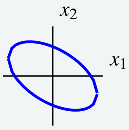
Use a change of variables to choose new axes such that the ellipse is oriented parallel to the new coordinate axes. In other words, use a change of variables to rewrite $q$ to eliminate the $x_1x_2$ term.
Solution 解
Notice that the level curve is given by $q = 7$ for $q = 6x_1^2 + 4x_1x_2 + 3x_2^2$. This is the same quadratic form that we examined earlier in Example $\PageIndex{13}$. Therefore we know that we can write $q = \vec{x}^T A \vec{x}$ for the matrix $A = \left[ \begin{array}{rr} 6 & 2 \\ 2 & 3 \end{array} \right] $$
Now we want to orthogonally diagonalize $A$ to write $U^TAU=D$ for an orthogonal matrix $U$ and diagonal matrix $D$. The details are left to the reader, and you can verify that the resulting matrices are $\begin{aligned} U &= \left[ \begin{array}{rr} \frac{2}{\sqrt{5}} & - \frac{1}{\sqrt{5}} \\ \frac{1}{\sqrt{5}} & \frac{2}{\sqrt{5}} \end{array} \right] $ D &= \left[ \begin{array}{rr} 7 & 0 \\ 0 & 2 \end{array} \right]\end{aligned}$$
Next we write $\vec{y} = \left[ \begin{array}{c} y_1 \\ y_2 \end{array} \right]$. It follows that $\vec{x} = U \vec{y}$.$
We can now express the quadratic form $q$ in terms of $y$, using the entries from $D$ as coefficients as follows: $\begin{aligned} q &= d\_{11}y_1^2 + d\_{22}y_2^2 \\ &= 7y_1^2 + 2y_2^2 \end{aligned}$$
Hence the level curve can be written $7y_1^2 + 2y_2^2 =7$. The graph of this equation is given by:
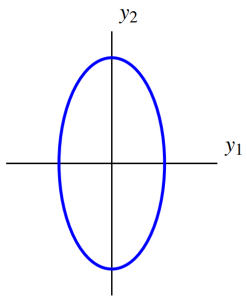
The change of variables results in new axes such that with respect to the new axes, the ellipse is oriented parallel to the coordinate axes. These are called the principal axes of the quadratic form.
The following is another example of diagonalizing a quadratic form.
Example 15: Choosing New Axes to Simplify a Quadratic Form 例 15:选取新坐标轴以化简二次型
Consider the level curve $5x_1^{2}-6x_1x_2+5x_2^{2}=8$ shown in the following graph.
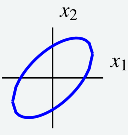
Use a change of variables to choose new axes such that the ellipse is oriented parallel to the new coordinate axes. In other words, use a change of variables to rewrite $q$ to eliminate the $x_1x_2$ term.
Solution 解
First, express the level curve as $\vec{x}^TA\vec{x}$ where $\vec{x} = \left[ \begin{array}{r} x_1 \\ x_2 \end{array} \right]$ and $A$ is symmetric. Let $A = \left[ \begin{array}{rr} a\_{11} & a\_{12} \\ a\_{21} & a\_{22} \end{array} \right]$. Then $q = \vec{x}^T A \vec{x}$ is given by $\begin{aligned} q &= \left[ \begin{array}{cc} x_1 & x_2 \end{array} \right] \left[ \begin{array}{rr} a\_{11} & a\_{12} \\ a\_{21} & a\_{22} \end{array} \right] \left[ \begin{array}{r} x_1 \\ x_2 \end{array} \right]$ &= a\_{11}x_1^2 + (a\_{12} + a\_{21})x_1x_2 + a\_{22}x_2^2\end{aligned}$$
Equating this to the given description for $q$, we have $5x_1^2 -6x_1x_2 + 5x_2^2 = a\_{11}x_1^2 + (a\_{12} + a\_{21})x_1x_2 + a\_{22}x_2^2 $ This implies that $a\_{11} = 5, a\_{22} = 5$ and in order for $A$ to be symmetric, $a\_{12} = a\_{22} = \frac{1}{2} (a\_{12}+a\_{21}) = -3$. The result is $A = \left[ \begin{array}{rr} 5 & -3 \\ -3 & 5 \end{array} \right]$. We can write $q = \vec{x}^TA\vec{x}$ as $\left[ \begin{array}{cc} x_1 & x_2 \end{array} \right] \left[ \begin{array}{rr} 5 & -3 \\ -3 & 5 \end{array} \right] \left[ \begin{array}{c} x_1 \\ x_2 \end{array} \right] =8 $$
Next, orthogonally diagonalize the matrix $A$ to write $U^TAU = D$. The details are left to the reader and the necessary matrices are given by $\begin{aligned} U &= \left[ \begin{array}{rr} \frac{1}{2}\sqrt{2} & \frac{1}{2}\sqrt{2} \\ \frac{1}{2}\sqrt{2} & - \frac{1}{2}\sqrt{2} \end{array} \right] $ D &= \left[ \begin{array}{rr} 2 & 0 \\ 0 & 8 \end{array} \right]\end{aligned}$$
Write $\vec{y} = \left[ \begin{array}{r} y_1 \\ y_2 \end{array} \right]$, such that $\vec{x} = U \vec{y}$. Then it follows that $q$ is given by $\begin{aligned} q &= d\_{11}y_1^2 + d\_{22}y_2^2 \\ &= 2y_1^{2}+8y_2^{2}\end{aligned}$ Therefore the level curve can be written as $2y_1^{2}+8y_2^{2}=8$.
This is an ellipse which is parallel to the coordinate axes. Its graph is of the form
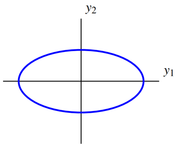
Thus this change of variables chooses new axes such that with respect to these new axes, the ellipse is oriented parallel to the coordinate axes.
Exercise 1 习题 1
If $A$ is an invertible $n\times n$ matrix, compare the eigenvalues of $A$ and $A^{−1}$. More generally, for $m$ an arbitrary integer, compare the eigenvalues of $A$ and $A^m$.
Answer $A^mX = λ^mX$ for any integer. In the case of $−1,$ A^{−1}λX = AA^{−1}X = X$ so $A^{−1}X = λ^{−1}X$. Thus the eigenvalues of $A^{−1}$ are just $λ^{-1}$ where $λ$ is an eigenvalue of $A$.
Exercise 2 习题 2
If $A$ is an $n\times n$ matrix and $c$ is a nonzero constant, compare the eigenvalues of $A$ and $cA$.
Answer Say $AX = λX$. Then $cAX = cλX$ and so the eigenvalues of $cA$ are just $cλ$ where $λ$ is an eigenvalue of $A$.
Exercise 3 习题 3
Let $A,$ B$ be invertible $n\times n$ matrices which commute. That is, $AB = BA$. Suppose $X$ is an eigenvector of $B$. Show that then $AX$ must also be an eigenvector for $B$.$
Answer $BAX = ABX = AλX = λAX$. Here it is assumed that $BX = λX$.
Exercise 4 习题 4
Suppose $A$ is an $n\times n$ matrix and it satisfies $A^m = A$ for some $m$ a positive integer larger than $1$. Show that if $λ$ is an eigenvalue of $A$ then $\|λ\|$ equals either $0$ or $1$.
Answer Let $X$ be the eigenvector. Then $A^mX = λ^mX,$ A^mX = AX = λX$ and so $\lambda^m=\lambda$ Hence if $\lambda\neq 0$, then $\lambda^{m-1}=1$ and so $\|\lambda\|=1$.$
Exercise 5 习题 5
Show that if $AX = λX$ and $AY = λY$, then whenever $k,$ p$ are scalars, $A(kX+pY)=\lambda (kX+pY)$ Does this imply that $kX+pY$ is an eigenvector? Explain.$
Answer The formula follows from properties of matrix multiplications. However, this vector might not be an eigenvector because it might equal $0$ and eigenvectors cannot equal $0$.
Exercise 6 习题 6
Suppose $A$ is a $3\times 3$ matrix and the following information is available. $\begin{aligned}A\left[\begin{array}{r}0&-1&-1\end{array}\right]&=0\left[\begin{array}{r}0&-1&-1\end{array}\right] $ A\left[\begin{array}{c}1&1&1\end{array}\right]&=-2\left[\begin{array}{c}1&1&1\end{array}\right] $ A\left[\begin{array}{r}-2&-3&-2\end{array}\right]&=-2\left[\begin{array}{r}-2&-3&-2\end{array}\right]\end{aligned}$ Find $A\left[\begin{array}{r}1&-4&3\end{array}\right]$.
Exercise 7 习题 7
Suppose $A$ is a $3\times 3$ matrix and the following information is available. $\begin{aligned}A\left[\begin{array}{r}-1&-2&-2\end{array}\right]&=1\left[\begin{array}{r}-1&-2&-2\end{array}\right] $ A\left[\begin{array}{c}1&1&1\end{array}\right]&=0\left[\begin{array}{c}1&1&1\end{array}\right] $ A\left[\begin{array}{r}-1&-4&-3\end{array}\right]&=2\left[\begin{array}{r}-1&-4&-3\end{array}\right]\end{aligned}$ Find $A\left[\begin{array}{r}3&-4&3\end{array}\right]$.
Exercise 8 习题 8
Suppose $A$ is a $3\times 3$ matrix and the following information is available. $\begin{aligned}A\left[\begin{array}{r}0&-1&-1\end{array}\right]&=2\left[\begin{array}{r}0&-1&-1\end{array}\right] $ A\left[\begin{array}{c}1&1&1\end{array}\right]&=1\left[\begin{array}{c}1&1&1\end{array}\right] $ A\left[\begin{array}{r}-3&-5&-4\end{array}\right]&=-3\left[\begin{array}{r}-3&-5&-4\end{array}\right]\end{aligned}$ Find $A\left[\begin{array}{r}2&-3&3\end{array}\right]$.
Exercise 9 习题 9
Find the eigenvalues and eigenvectors of the matrix $\left[\begin{array}{rrr}-6&-92&12 \\ 0&0&0&-2&-31&4\end{array}\right]$ One eigenvalue is $-2$.
Exercise 10 习题 10
Find the eigenvalues and eigenvectors of the matrix $\left[\begin{array}{rrr}-2&-17&-6 \\ 0&0&0&1&9&3\end{array}\right]$ One eigenvalue is $1$.
Exercise 11 习题 11
Find the eigenvalues and eigenvectors of the matrix $\left[\begin{array}{rrr}9&2&8 \\ 2&-6&-2 \\ -8&2&-5\end{array}\right]$ One eigenvalue is $-3$.
Exercise 12 习题 12
Find the eigenvalues and eigenvectors of the matrix $\left[\begin{array}{rrr}6&76&16 \\ -2&-21&-4 \\ 2&64&17\end{array}\right]$ One eigenvalue is $-2$.
Exercise 13 习题 13
Find the eigenvalues and eigenvectors of the matrix $\left[\begin{array}{rrr}3&5&2 \\ -8&-11&-4 \\ 10&11&3\end{array}\right]$ One eigenvalue is $-3$.
Exercise 14 习题 14
Is it possible for a nonzero matrix to have only $0$ as an eigenvalue?
Answer Yes. $\left[\begin{array}{cc}0&1&0&0\end{array}\right]$ works.$
Exercise 15 习题 15
If $A$ is the matrix of a linear transformation which rotates all vectors in $\mathbb{R}^2$ through $60^{\circ}$, explain why $A$ cannot have any real eigenvalues. Is there an angle such that rotation through this angle would have a real eigenvalue? What eigenvalues would be obtainable in this way?
Exercise 16 习题 16
Let $A$ be the $2\times 2$ matrix of the linear transformation which rotates all vectors in $\mathbb{R}^2$ through an angle of $θ$. For which values of $θ$ does $A$ have a real eigenvalue?
Answer When you think of this geometrically, it is clear that the only two values of $θ$ are $0$ and $π$ or these added to integer multiples of $2π$.
Exercise 17 习题 17
Let $T$ be the linear transformation which reflects vectors about the $x$ axis. Find a matrix for $T$ and then find its eigenvalues and eigenvectors.
Answer The matrix of $T$ is $\left[\begin{array}{rr}1&0&0&-1\end{array}\right]$. The eigenvectors and eigenvalues are: $\left\{left$$\begin{array}{c}0&1\end{array}\right]\right\}↔ -1,$\left\{left$$\begin{array}{c}1&0\end{array}\right]\right\}↔1$
Exercise 18 习题 18
Let $T$ be the linear transformation which rotates all vectors in $\mathbb{R}^2$ counterclockwise through an angle of $π/2$. Find a matrix of $T$ and then find eigenvalues and eigenvectors.
Answer The matrix of $T$ is $\left[\begin{array}{rr}0&-1&1&0\end{array}\right]$. The eigenvectors and eigenvalues are: $\left\{left$$\begin{array}{c}-i&1\end{array}\right]\right\}↔ -i,$\left\{left$$\begin{array}{c}i&1\end{array}\right]\right\}↔i$
Exercise 19 习题 19
Let $T$ be the linear transformation which reflects all vectors in $\mathbb{R}^3$ through the $xy$ plane. Find a matrix for $T$ and then obtain its eigenvalues and eigenvectors.
Answer The matrix of $T$ is $\left[\begin{array}{ccc}1&0&0&0&1&0&0&0&-1\end{array}\right]$. The eigenvectors and eigenvalues are: $\left\{left$$\begin{array}{c}0&0&1\end{array}\right]\right\}↔-1,$\left\{left$$\begin{array}{c}1&0&0\end{array}\right],$\left[\begin{array}{c}0&1&0\end{array}\right]\right\}↔1$
Exercise 20 习题 20
Find the eigenvalues and eigenvectors of the matrix $\left[\begin{array}{rrr}5&-18&-32&0&5&4&2&-5&-11\end{array}\right]$ One eigenvalue is $1$. Diagonalize if possible.
Answer The eigenvalues are $−1,−1, 1$. The eigenvectors corresponding to the eigenvalues are: $\left\{left$$\begin{array}{r}10&-2&3\end{array}\right]\right\}↔-1,$\left\{left$$\begin{array}{r}7&-2&2\end{array}\right]\right\}↔1$ Therefore this matrix is not diagonalizable.$
Exercise 21 习题 21
Find the eigenvalues and eigenvectors of the matrix $\left[\begin{array}{rrr}-12&-28&28&4&9&-8&-4&-8&9\end{array}\right]$ One eigenvalue is $3$. Diagonalize if possible.
Answer The eigenvectors and eigenvalues are: $\left\{left$$\begin{array}{c}2&0&1\end{array}\right]\right\}↔1,$\left\{left$$\begin{array}{r}-2&1&0\end{array}\right]\right\}↔1,$\left\{left$$\begin{array}{r}7&-2&2\end{array}\right]\right\}↔3$ The matrix $P$ needed to diagonalize the above matrix is $\left[\begin{array}{rrr}2&-2&7&0&1&-2&1&0&2\end{array}\right]$ and the diagonal matrix $D$ is $\left[\begin{array}{ccc}1&0&0&0&1&0&0&0&3\end{array}\right]$
Exercise 22 习题 22
Find the eigenvalues and eigenvectors of the matrix $\left[\begin{array}{rrr}89&38&268&14&2&40&-30&-12&-90\end{array}\right]$ One eigenvalue is $-3$. Diagonalize if possible.
Answer The eigenvectors and eigenvalues are: $\left\{left$$\begin{array}{c}-6&-1&-2\end{array}\right]\right\}↔6,$\left\{left$$\begin{array}{r}-5&-2&2\end{array}\right]\right\}↔-3,$\left\{left$$\begin{array}{r}-8&-2&3\end{array}\right]\right\}↔2$ The matrix $P$ needed to diagonalize the above matrix is $\left[\begin{array}{rrr}-6&-5&-8&-1&-2&-2&2&2&3\end{array}\right]$ and the diagonal matrix $D$ is $\left[\begin{array}{rrr}6&0&0&0&-3&0&0&0&-2\end{array}\right]$
Exercise 23 习题 23
Find the eigenvalues and eigenvectors of the matrix $\left[\begin{array}{rrr}1&90&0&0&-2&0&3&89&-2\end{array}\right]$ One eigenvalue is $1$. Diagonalize if possible.
Exercise 24 习题 24
Find the eigenvalues and eigenvectors of the matrix $\left[\begin{array}{rrr}11&45&30&10&26&20&-20&-60&-44\end{array}\right]$ One eigenvalue is $1$. Diagonalize if possible.
Exercise 25 习题 25
Find the eigenvalues and eigenvectors of the matrix $\left[\begin{array}{rrr}95&25&24&-196&-53&-48&-164&-42&-43\end{array}\right]$ One eigenvalue is $5$. Diagonalize if possible.
Exercise 26 习题 26
Suppose $A$ is an $n\times n$ matrix and let $V$ be an eigenvector such that $AV = λV$. Also suppose the characteristic polynomial of $A$ is $\det (xI-A)=x^n+a\_{n-1}x^{n-1}+\cdots +a_1x+a_0$ Explain why \$A^n+a\_{n-1}A^{n-1}+\cdots +a_1A+a_0I)V=0$ If $A$ is diagonalizable, give a proof of the Cayley Hamilton theorem based on this. This theorem says $A$ satisfies its characteristic equation $A^n+a\_{n-1}A^{n-1}+\cdots +a_1A+a_0I=0$$
Exercise 27 习题 27
Suppose the characteristic polynomial of an $n\times n$ matrix $A$ is $1−X^n$. Find $A^{mn}$ where $m$ is an integer.
Answer The eigenvalues are distinct because they are the $n$th roots of $1$. Hence if $X$ is a given vector with $X=\sum\limits\_{j=1}^na_jV_j$ then $A^{nm}X=A^{nm}\sum\limits\_{j=1}^na_jV_j=\sum\limits\_{j=1}^na_jA^{nm}V_j=\sum\limits\_{j=1}^na_jV_j=X$ so $A^{nm}=I$.
Exercise 28 习题 28
Find the eigenvalues and eigenvectors of the matrix $\left[\begin{array}{rrr}15&-24&7&-6&5&-1&-58&76&-20\end{array}\right]$ One eigenvalue is $−2$. Diagonalize if possible. Hint: This one has some complex eigenvalues.
Exercise 29 习题 29
Find the eigenvalues and eigenvectors of the matrix $\left[\begin{array}{rrr}15&-25&6&-13&23&-4&-91&155&-30\end{array}\right]$ One eigenvalue is $2$. Diagonalize if possible. Hint: This one has some complex eigenvalues.
Exercise 30 习题 30
Find the eigenvalues and eigenvectors of the matrix $\left[\begin{array}{rrr}-11&-12&4&8&17&-4&-4&28&-3\end{array}\right]$ One eigenvalue is $1$. Diagonalize if possible. Hint: This one has some complex eigenvalues.
Exercise 31 习题 31
Find the eigenvalues and eigenvectors of the matrix $\left[\begin{array}{rrr}14&-12&5&-6&2&-1&-69&51&-21\end{array}\right]$ One eigenvalue is $−3$. Diagonalize if possible. Hint: This one has some complex eigenvalues.
Exercise 32 习题 32
Suppose $A$ is an $n\times n$ matrix consisting entirely of real entries but $a + ib$ is a complex eigenvalue having the eigenvector, $X +iY$ Here $X$ and $Y$ are real vectors. Show that then $a−ib$ is also an eigenvalue with the eigenvector, $X − iY$. Hint: You should remember that the conjugate of a product of complex numbers equals the product of the conjugates. Here $a+ib$ is a complex number whose conjugate equals $a−ib$.
Answer
$$AX = (a+ib)X\\. Now take conjugates of both sides. Since \\A\\ is real, \\A\overline{X}=(a-ib)\overline{X}$$
Exercise 33 习题 33
Let $A=\left[\begin{array}{cc}1&2&2&1\end{array}\right]$. Diagonalize $A$ to find $A^{10}$.$
Answer
First we write $A=PDP^{-1}$. $\left[\begin{array}{cc}1&2&2&1\end{array}\right]=\left[\begin{array}{rr}-1&1&1&1\end{array}\right]\left[\begin{array}{rr}-1&0&0&3\end{array}\right]=\left[\begin{array}{rr}-\frac{1}{2}&\frac{1}{2} \\ \frac{1}{2}&\frac{1}{2}\end{array}\right]$ Therefore $A^{10}=PD^{10}P^{-1}$. $\begin{aligned}\left[\begin{array}{cc}1&2&2&1\end{array}\right]^{10}&=\left[\begin{array}{rr}-1&1&1&1\end{array}\right]\left[\begin{array}{rr}-1&0&0&3\end{array}\right]^{10}\left[\begin{array}{rr}-\frac{1}{2}&\frac{1}{2}& \frac{1}{2}&\frac{1}{2}\end{array}\right] $ &=\left[\begin{array}{rr}-1&1&1&1\end{array}\right]\left[\begin{array}{rr}(-1)^{10}&0&0&3^{10}\end{array}\right]\left[\begin{array}{rr}-\frac{1}{2}&\frac{1}{2}& \frac{1}{2}&\frac{1}{2}\end{array}\right] $ &=\left[\begin{array}{rr}29525&29524 \\ 29524&29525\end{array}\right]\end{aligned}$
Exercise 34 习题 34
Let $A=\left[\begin{array}{ccc}1&4&1&0&2&5&0&0&5\end{array}\right]$. Diagonalize $A$ to find $A^{50}$.
Exercise 35 习题 35
Let $A=\left[\begin{array}{rrr}1&-2&-1&2&-1&1&-2&3&1\end{array}\right]$. Diagonalize $A$ to find $A^{100}$.
Exercise 36 习题 36
The following is a Markov (migration) matrix for three locations $\left[\begin{array}{ccc}\frac{7}{10}&\frac{1}{9}&\frac{1}{5} \\ \frac{1}{10}&\frac{7}{9}&\frac{2}{5} \\ \frac{1}{5}&\frac{1}{9}&\frac{2}{5}\end{array}\right]$
- Initially, there are $90$ people in location $1,$ 81$ in location $2$, and $85$ in location $3$. How many are in each location after one time period?$
- The total number of individuals in the migration process is $256$. After a long time, how many are in each location?
- 初始时地点 $1$ 有 $90$ 人,地点 $2$ 有 $81$ 人,地点 $3$ 有 $85$ 人。经过一个时间周期后,各地各有多少人?
- 迁移过程中总人数为 $256$。经过足够长时间后,各地各有多少人?
Answer
- Multiply the given matrix by the initial state vector given by $\left[\begin{array}{c}90&81&85\end{array}\right]$. After one time period there are $89$ people in location $1$, $106$ in location $2$, and $61$ in location $3$.
- Solve the system given by \$I − A)X_s = 0$ where $A$ is the migration matrix and $X_s=\left[\begin{array}{c}x\_{1s} \\ x\_{2s} \\ x\_{3s}\end{array}\right]$ is the steady state vector. The solution to this system is given by $\begin{aligned}x\_{1s}&=\frac{8}{5}x\_{3s} \\ x\_{2s}&=\frac{63}{25}x\_{3s}\end{aligned}$ Letting $x\_{3s} = t$ and using the fact that there are a total of $256$ individuals, we must solve $\frac{8}{5}t+\frac{63}{25}t+t=256$ We find that $t = 50$. Therefore after a long time, there are $80$ people in location $1,$ 126$ in location $2$, and $50$ in location $3$.$
- 将给定的矩阵乘以初始状态向量 $\left[\begin{array}{c}90&81&85\end{array}\right]$。经过一个时间周期后,地点 $1$ 有 $89$ 人,地点 $2$ 有 $106$ 人,地点 $3$ 有 $61$ 人。
- 对稳态向量 $X_s=\left[\begin{array}{c}x_{1s} \\ x_{2s} \\ x_{3s}\end{array}\right]$ 求解方程组 $(I-A)X_s = 0$,其中 $A$ 为迁移矩阵。该方程组的解为 $\begin{aligned}x_{1s}&=\frac{8}{5}x_{3s} \\ x_{2s}&=\frac{63}{25}x_{3s}\end{aligned}$。令 $x_{3s} = t$,并由总人数为 $256$,须解 $\frac{8}{5}t+\frac{63}{25}t+t=256$,得 $t = 50$。因此经过足够长时间后,地点 $1$ 有 $80$ 人,地点 $2$ 有 $126$ 人,地点 $3$ 有 $50$ 人。
Exercise 37 习题 37
The following is a Markov (migration) matrix for three locations $\left[\begin{array}{ccc}\frac{1}{5}&\frac{1}{5}&\frac{2}{5} \\ \frac{2}{5}&\frac{2}{5}&\frac{1}{5} \\ \frac{2}{5}&\frac{2}{5}&\frac{2}{5}\end{array}\right]$
- Initially, there are $130$ individuals in location $1,$ 300$ in location $2$, and $70$ in location $3$. How many are in each location after two time periods?$
- The total number of individuals in the migration process is $500$. After a long time, how many are in each location?
- 初始时地点 $1$ 有 $130$ 人,地点 $2$ 有 $300$ 人,地点 $3$ 有 $70$ 人。经过两个时间周期后,各地各有多少人?
- 迁移过程中总人数为 $500$。经过足够长时间后,各地各有多少人?
Exercise 38 习题 38
The following is a Markov (migration) matrix for three locations $\left[\begin{array}{ccc}\frac{3}{10}&\frac{3}{8}&\frac{1}{3} \\ \frac{1}{10}&\frac{3}{8}&\frac{1}{3} \\ \frac{3}{5}&\frac{1}{4}&\frac{1}{3}\end{array}\right]$ The total number of individuals in the migration process is $480$. After a long time, how many are in each location?
Answer
We solve \$I −A)X_s = 0$ to find the steady state vector $X_s=\left[\begin{array}{c}x\_{1s} \\ x\_{2s} \\ x\_{3s}\end{array}\right]$. The solution to the system is given by $\begin{aligned}x\_{1s}&=\frac{5}{6}x\_{3s} \\ x\_{2s}&=\frac{2}{3}x\_{3s}\end{aligned}$ Letting $x\_{3s} = t$ and using the fact that there are a total of $480$ individuals, we must solve $\frac{5}{6}t+\frac{2}{3}t+t=480$ We find that $t = 192$. Therefore after a long time, there are $160$ people in location $1,$ 128$ in location $2$, and $192$ in location $3$.$
Exercise 39 习题 39
The following is a Markov (migration) matrix for three locations $\left[\begin{array}{ccc}\frac{3}{10}&\frac{1}{3}&\frac{1}{5} \\ \frac{3}{10}&\frac{1}{3}&\frac{7}{10} \\ \frac{2}{5}&\frac{1}{3}&\frac{1}{10}\end{array}\right]$ The total number of individuals in the migration process is $1155$. After a long time, how many are in each location?
Exercise 40 习题 40
The following is a Markov (migration) matrix for three locations $\left[\begin{array}{ccc}\frac{2}{5}&\frac{1}{10}&\frac{1}{8} \\ \frac{3}{10}&\frac{2}{5}&\frac{5}{8} \\ \frac{3}{10}&\frac{1}{2}&\frac{1}{4}\end{array}\right]$ The total number of individuals in the migration process is $704$. After a long time, how many are in each location?
Exercise 41 习题 41
A person sets off on a random walk with three possible locations. The Markov matrix of probabilities $A = $$a\_{ij}$$$ is given by $\left[\begin{array}{ccc}0.1&0.3&0.7 \\ 0.1&0.3&0.2&0.8&0.4&0.1\end{array}\right]$ If the walker starts in location $2$, what is the probability of ending back in location $2$ at time $n = 3$?
Answer
$X_3=\left[\begin{array}{c}0.38&0.18&0.44\end{array}\right]$ Therefore the probability of ending up back in location $2$ is $0.18$.
Exercise 42 习题 42
A person sets off on a random walk with three possible locations. The Markov matrix of probabilities $A = $$a\_{ij}$$$ is given by $\left[\begin{array}{ccc}0.5&0.1&0.6&0.2&0.9&0.2&0.3&0&0.2\end{array}\right]$ It is unknown where the walker starts, but the probability of starting in each location is given by $X_0=\left[\begin{array}{r}0.2&0.25&0.55\end{array}\right]$ What is the probability of the walker being in location $1$ at time $n = 2$?
Answer
$X_2=\left[\begin{array}{r}0.367&0.4625&0.1705\end{array}\right]$ Therefore the probability of ending up in location $1$ is $0.367$.
Exercise 43 习题 43
You own a trailer rental company in a large city and you have four locations, one in the South East, one in the North East, one in the North West, and one in the South West. Denote these locations by SE, NE, NW, and SW respectively. Suppose that the following table is observed to take place.
| SE | NE | NW | SW | |
|---|---|---|---|---|
| SE | $\frac{1}{3}$ | $\frac{1}{10}$ | $\frac{1}{10}$ | $\frac{1}{5}$ |
| NE | $\frac{1}{3}$ | $\frac{7}{10}$ | $\frac{1}{5}$ | $\frac{1}{10}$ |
| NW | $\frac{2}{9}$ | $\frac{1}{10}$ | $\frac{3}{5}$ | $\frac{1}{5}$ |
| SW | $\frac{1}{9}$ | $\frac{1}{10}$ | $\frac{1}{10}$ | $\frac{1}{2}$ |
| 东南 | 东北 | 西北 | 西南 | |
|---|---|---|---|---|
| 东南 | $\frac{1}{3}$ | $\frac{1}{10}$ | $\frac{1}{10}$ | $\frac{1}{5}$ |
| 东北 | $\frac{1}{3}$ | $\frac{7}{10}$ | $\frac{1}{5}$ | $\frac{1}{10}$ |
| 西北 | $\frac{2}{9}$ | $\frac{1}{10}$ | $\frac{3}{5}$ | $\frac{1}{5}$ |
| 西南 | $\frac{1}{9}$ | $\frac{1}{10}$ | $\frac{1}{10}$ | $\frac{1}{2}$ |
Table PageIndex 1
In this table, the probability that a trailer starting at NE ends in NW is $1/10$, the probability that a trailer starting at SW ends in NW is $1/5$, and so forth. Approximately how many will you have in each location after a long time if the total number of trailers is $413$?
Answer
The migration matrix is $A=\left[\begin{array}{cccc}\frac{1}{3}&\frac{1}{10}&\frac{1}{10}&\frac{1}{5} \\ \frac{1}{3}&\frac{7}{10}&\frac{1}{5}&\frac{1}{10} \\ \frac{2}{9}&\frac{1}{10}&\frac{3}{5}&\frac{1}{5} \\ \frac{1}{9}&\frac{1}{10}&\frac{1}{10}&\frac{1}{2}\end{array}\right]$ To find the number of trailers in each location after a long time we solve system \$I − A)X_s = 0$ for the steady state vector $X_s=\left[\begin{array}{c}x\_{1s} \\ x\_{2s} \\ x\_{3s} \\ x\_{4s}\end{array}\right]$. The solution to this system is $\begin{aligned} x\_{1s}&=\frac{9}{10}x\_{4s} \\ x\_{2s}&=\frac{12}{5}x\_{4s} \\ x\_{3s}&=\frac{8}{5}x\_{4s}\end{aligned}$ Letting $x\_{4s} = t$ and using the fact that there are a total of $413$ trailers we must solve $\frac{9}{10}t+\frac{12}{5}t+\frac{8}{5}t+t=413$ We find that $t = 70$. Therefore after a long time, there are $63$ trailers in the SE, $168$ in the NE, $112$ in the NW and $70$ in the SW.$
Exercise 44 习题 44
You own a trailer rental company in a large city and you have four locations, one in the South East, one in the North East, one in the North West, and one in the South West. Denote these locations by SE, NE, NW, and SW respectively. Suppose that the following table is observed to take place.
| SE | NE | NW | SW | |
|---|---|---|---|---|
| SE | $\frac{1}{7}$ | $\frac{1}{4}$ | $\frac{1}{10}$ | $\frac{1}{5}$ |
| NE | $\frac{2}{7}$ | $\frac{1}{4}$ | $\frac{1}{5}$ | $\frac{1}{10}$ |
| NW | $\frac{1}{7}$ | $\frac{1}{4}$ | $\frac{3}{5}$ | $\frac{1}{5}$ |
| SW | $\frac{3}{7}$ | $\frac{1}{4}$ | $\frac{1}{10}$ | $\frac{1}{2}$ |
| 东南 | 东北 | 西北 | 西南 | |
|---|---|---|---|---|
| 东南 | $\frac{1}{7}$ | $\frac{1}{4}$ | $\frac{1}{10}$ | $\frac{1}{5}$ |
| 东北 | $\frac{2}{7}$ | $\frac{1}{4}$ | $\frac{1}{5}$ | $\frac{1}{10}$ |
| 西北 | $\frac{1}{7}$ | $\frac{1}{4}$ | $\frac{3}{5}$ | $\frac{1}{5}$ |
| 西南 | $\frac{3}{7}$ | $\frac{1}{4}$ | $\frac{1}{10}$ | $\frac{1}{2}$ |
Table PageIndex 2
In this table, the probability that a trailer starting at NE ends in NW is 1/10, the probability that a trailer starting at SW ends in NW is 1/5, and so forth. Approximately how many will you have in each location after a long time if the total number of trailers is 1469.
Exercise 45 习题 45
The following table describes the transition probabilities between the states rainy, partly cloudy and sunny. The symbol p.c. indicates partly cloudy. Thus if it starts off p.c. it ends up sunny the next day with probability $\frac{1}{5}$. If it starts off sunny, it ends up sunny the next day with probability $\frac{2}{5}$ and so forth.
| rains | sunny | p.c. | |
|---|---|---|---|
| rains | $\frac{1}{5}$ | $\frac{1}{5}$ | $\frac{1}{3}$ |
| sunny | $\frac{1}{5}$ | $\frac{2}{5}$ | $\frac{1}{3}$ |
| p.c. | $\frac{3}{5}$ | $\frac{2}{5}$ | $\frac{1}{3}$ |
| 雨 | 晴 | 局部多云 | |
|---|---|---|---|
| 雨 | $\frac{1}{5}$ | $\frac{1}{5}$ | $\frac{1}{3}$ |
| 晴 | $\frac{1}{5}$ | $\frac{2}{5}$ | $\frac{1}{3}$ |
| 局部多云 | $\frac{3}{5}$ | $\frac{2}{5}$ | $\frac{1}{3}$ |
Table PageIndex 3
Given this information, what are the probabilities that a given day is rainy, sunny, or partly cloudy?
Exercise 46 习题 46
The following table describes the transition probabilities between the states rainy, partly cloudy and sunny. The symbol p.c. indicates partly cloudy. Thus if it starts off p.c. it ends up sunny the next day with probability $\frac{1}{10}$. If it starts off sunny, it ends up sunny the next day with probability $\frac{2}{5}$ and so forth.
| rains | sunny | p.c. | |
|---|---|---|---|
| rains | $\frac{1}{5}$ | $\frac{1}{5}$ | $\frac{1}{3}$ |
| sunny | $\frac{1}{10}$ | $\frac{2}{5}$ | $\frac{4}{9}$ |
| p.c. | $\frac{7}{10}$ | $\frac{2}{5}$ | $\frac{2}{9}$ |
| 雨 | 晴 | 局部多云 | |
|---|---|---|---|
| 雨 | $\frac{1}{5}$ | $\frac{1}{5}$ | $\frac{1}{3}$ |
| 晴 | $\frac{1}{10}$ | $\frac{2}{5}$ | $\frac{4}{9}$ |
| 局部多云 | $\frac{7}{10}$ | $\frac{2}{5}$ | $\frac{2}{9}$ |
Table PageIndex 4
Given this information, what are the probabilities that a given day is rainy, sunny, or partly cloudy?
Exercise 47 习题 47
You own a trailer rental company in a large city and you have four locations, one in the South East, one in the North East, one in the North West, and one in the South West. Denote these locations by SE, NE, NW, and SW respectively. Suppose that the following table is observed to take place.
| SE | NE | NW | SW | |
|---|---|---|---|---|
| SE | $\frac{5}{11}$ | $\frac{1}{10}$ | $\frac{1}{10}$ | $\frac{1}{5}$ |
| NE | $\frac{1}{11}$ | $\frac{7}{10}$ | $\frac{1}{5}$ | $\frac{1}{10}$ |
| NW | $\frac{2}{11}$ | $\frac{1}{10}$ | $\frac{3}{5}$ | $\frac{1}{5}$ |
| SW | $\frac{3}{11}$ | $\frac{1}{10}$ | $\frac{1}{10}$ | $\frac{1}{2}$ |
| 东南 | 东北 | 西北 | 西南 | |
|---|---|---|---|---|
| 东南 | $\frac{5}{11}$ | $\frac{1}{10}$ | $\frac{1}{10}$ | $\frac{1}{5}$ |
| 东北 | $\frac{1}{11}$ | $\frac{7}{10}$ | $\frac{1}{5}$ | $\frac{1}{10}$ |
| 西北 | $\frac{2}{11}$ | $\frac{1}{10}$ | $\frac{3}{5}$ | $\frac{1}{5}$ |
| 西南 | $\frac{3}{11}$ | $\frac{1}{10}$ | $\frac{1}{10}$ | $\frac{1}{2}$ |
Table PageIndex 5
In this table, the probability that a trailer starting at NE ends in NW is 1/10, the probability that a trailer starting at SW ends in NW is 1/5, and so forth. Approximately how many will you have in each location after a long time if the total number of trailers is 407?
Exercise 48 习题 48
The University of Poohbah offers three degree programs, scouting education (SE), dance appreciation (DA), and engineering (E). It has been determined that the probabilities of transferring from one program to another are as in the following table.
| SE | DA | E | |
|---|---|---|---|
| SE | $.8$ | $.1$ | $.3$ |
| DA | $.1$ | $.7$ | $.5$ |
| E | $.1$ | $.2$ | $.2$ |
| 童子军教育 | 舞蹈鉴赏 | 工程 | |
|---|---|---|---|
| 童子军教育 | $.8$ | $.1$ | $.3$ |
| 舞蹈鉴赏 | $.1$ | $.7$ | $.5$ |
| 工程 | $.1$ | $.2$ | $.2$ |
Table PageIndex 6
where the number indicates the probability of transferring from the top program to the program on the left. Thus the probability of going from DA to E is $.2$. Find the probability that a student is enrolled in the various programs.
Exercise 49 习题 49
In the city of Nabal, there are three political persuasions, republicans (R), democrats (D), and neither one (N). The following table shows the transition probabilities between the political parties, the top row being the initial political party and the side row being the political affiliation the following year.
| R | D | N | |
|---|---|---|---|
| R | $\frac{1}{5}$ | $\frac{1}{6}$ | $\frac{2}{7}$ |
| D | $\frac{1}{5}$ | $\frac{1}{3}$ | $\frac{4}{7}$ |
| N | $\frac{3}{5}$ | $\frac{1}{2}$ | $\frac{1}{7}$ |
| 共和党 | 民主党 | 无党派 | |
|---|---|---|---|
| 共和党 | $\frac{1}{5}$ | $\frac{1}{6}$ | $\frac{2}{7}$ |
| 民主党 | $\frac{1}{5}$ | $\frac{1}{3}$ | $\frac{4}{7}$ |
| 无党派 | $\frac{3}{5}$ | $\frac{1}{2}$ | $\frac{1}{7}$ |
Table PageIndex 7
Find the probabilities that a person will be identified with the various political persuasions. Which party will end up being most important?
Exercise 50 习题 50
The following table describes the transition probabilities between the states rainy, partly cloudy and sunny. The symbol p.c. indicates partly cloudy. Thus if it starts off p.c. it ends up sunny the next day with probability $\frac{1}{5}$. If it starts off sunny, it ends up sunny the next day with probability $\frac{2}{7}$ and so forth.
| rains | sunny | p.c. | |
|---|---|---|---|
| rains | $\frac{1}{5}$ | $\frac{2}{7}$ | $\frac{5}{9}$ |
| sunny | $\frac{1}{5}$ | $\frac{2}{7}$ | $\frac{1}{3}$ |
| p.c. | $\frac{3}{5}$ | $\frac{3}{7}$ | $\frac{1}{9}$ |
| 雨 | 晴 | 局部多云 | |
|---|---|---|---|
| 雨 | $\frac{1}{5}$ | $\frac{2}{7}$ | $\frac{5}{9}$ |
| 晴 | $\frac{1}{5}$ | $\frac{2}{7}$ | $\frac{1}{3}$ |
| 局部多云 | $\frac{3}{5}$ | $\frac{3}{7}$ | $\frac{1}{9}$ |
Table PageIndex 8
Given this information, what are the probabilities that a given day is rainy, sunny, or partly cloudy?
Exercise 51 习题 51
Find the solution to the initial value problem $\begin{aligned}\left[\begin{array}{c}x&y\end{array}\right]'&=\left[\begin{array}{rr}0&-1&6&5\end{array}\right]\left[\begin{array}{c}x&y\end{array}\right]$ \left[\begin{array}{c}x(0) \\ y(0)\end{array}\right]&=\left[\begin{array}{c}2&2\end{array}\right]\end{aligned}$ Hint: form the matrix exponential $e^{At}$ and then the solution is $e^{At}C$ where $C$ is the initial vector,
Answer
The solution is $e^{At}C=\left[\begin{array}{c}8e^{2t}-6e^{3t} \\ 18e^{3t}-16e^{2t}\end{array}\right]$
Exercise 52 习题 52
Find the solution to the initial value problem $\begin{aligned}\left[\begin{array}{c}x&y\end{array}\right]'&=\left[\begin{array}{rr}-4&-3&6&5\end{array}\right]\left[\begin{array}{c}x&y\end{array}\right]$ \left[\begin{array}{c}x(0) \\ y(0)\end{array}\right]&=\left[\begin{array}{c}3&4\end{array}\right]\end{aligned}$ Hint: form the matrix exponential $e^{At}$ and then the solution is $e^{At}C$ where $C$ is the initial vector.
Exercise 53 习题 53
Exercise 54 习题 54
Find the eigenvalues and an orthonormal basis of eigenvectors for $A$. $A=\left[\begin{array}{rrr}11&-1&-4 \\ -1&11&-4&-4&-4&14\end{array}\right]$ Hint: Two eigenvalues are $12$ and $18$.
Answer. The eigenvectors and eigenvalues are: $\left\{frac{1}{\sqrt{3}}\left[\begin{array}{c}1&1&1\end{array}\right]\right\}leftrightarrow 6,\left\{frac{1}{\sqrt{2}}\left[\begin{array}{r}-1&1&0\end{array}\right]\right\}leftrightarrow 12,\left\{frac{1}{\sqrt{6}}\left[\begin{array}{r}-1&-1&2\end{array}\right]\right\}leftrightarrow 18$
Exercise 55 习题 55
Find the eigenvalues and an orthonormal basis of eigenvectors for $A$. $A=\left[\begin{array}{rrr}4&1&-2&1&4&-2&-2&-2&7\end{array}\right]$ Hint: One eigenvalue is $3$.
Answer. The eigenvectors and eigenvalues are: $\left\{frac{1}{\sqrt{2}}\left[\begin{array}{r}-1&1&0\end{array}\right],\frac{1}{\sqrt{3}}\left[\begin{array}{c}1&1&1\end{array}\right]\right\}leftrightarrow 3,\left\{frac{1}{\sqrt{6}}\left[\begin{array}{r}-1&-1&2\end{array}\right]\right\}leftrightarrow 9$
Exercise 56 习题 56
Find the eigenvalues and an orthonormal basis of eigenvectors for $A$. Diagonalize $A$ by finding an orthogonal matrix $U$ and a diagonal matrix $D$ such that $U^TAU = D$. $A=\left[\begin{array}{rrr}-1&1&1&1&-1&1&1&1&-1\end{array}\right]$ Hint: One eigenvalue is $-2$.
Answer. The eigenvectors and eigenvalues are: $\left\{left$$\begin{array}{c}\frac{1}{3}\sqrt{3} \\ \frac{1}{3}\sqrt{3} \\ \frac{1}{3}\sqrt{3}\end{array}\right]\right\}leftrightarrow 1,\left\{left$$\begin{array}{c}-\frac{1}{2}\sqrt{2} \\ \frac{1}{2}\sqrt{2} \\ 0\end{array}\right],\left[\begin{array}{c}-\frac{1}{6}\sqrt{6} \\ -\frac{1}{6}\sqrt{6} \\ \frac{1}{3}\sqrt{2}\sqrt{3}\end{array}\right]\right\}leftrightarrow -2$ $\left[\begin{array}{c}\sqrt{3}/3&-\sqrt{2}/2&-\sqrt{6}/6 \\ \sqrt{3}/3&\sqrt{2}/2&-\sqrt{6}/6 \\ \sqrt{3}/3&0&\frac{1}{3}\sqrt{2}\sqrt{3}\end{array}\right]^T\left[\begin{array}{rrr}-1&1&1&1&-1&1&1&1&-1\end{array}\right]$ $\left[\begin{array}{c}\sqrt{3}/3&-\sqrt{2}/2&-\sqrt{6}/6 \\ \sqrt{3}/3&\sqrt{2}/2&-\sqrt{6}/6 \\ \sqrt{3}/3&0&\frac{1}{3}\sqrt{2}\sqrt{3}\end{array}\right]$ $=\left[\begin{array}{rrr}1&0&0&0&-2&0&0&0&-2\end{array}\right]$
Exercise 57 习题 57
Find the eigenvalues and an orthonormal basis of eigenvectors for $A$. Diagonalize $A$ by finding an orthogonal matrix $U$ and a diagonal matrix $D$ such that $U^TAU = D$. $A=\left[\begin{array}{rrr}17&-7&-4 \\ -7&17&-4 \\ -4&-4&14\end{array}\right]$ Hint: Two eigenvalues are $18$ and $24$.
Answer. The eigenvectors and eigenvalues are: $\left\{left$$\begin{array}{c}\frac{1}{3}\sqrt{3} \\ \frac{1}{3}\sqrt{3} \\ \frac{1}{3}\sqrt{3}\end{array}\right]\right\}leftrightarrow 6,\left\{left$$\begin{array}{c}-\frac{1}{6}\sqrt{6} \\ -\frac{1}{6}\sqrt{6} \\ \frac{1}{3}\sqrt{2}\sqrt{3}\end{array}\right]\right\}leftrightarrow 18,\left\{left$$\begin{array}{c}-\frac{1}{2}\sqrt{2} \\ \frac{1}{2}\sqrt{2} \\ 0\end{array}\right]\right\}leftrightarrow 24$ The matrix $U$ has these as its columns.
Exercise 58 习题 58
Find the eigenvalues and an orthonormal basis of eigenvectors for $A$. Diagonalize $A$ by finding an orthogonal matrix $U$ and a diagonal matrix $D$ such that $U^TAU = D$. $A=\left[\begin{array}{rrr}13&1&4&1&13&4&4&4&10\end{array}\right]$ Hint: Two eigenvalues are $12$ and $18$.
Answer. The eigenvectors and eigenvalues are: $\left\{left$$\begin{array}{c}-\frac{1}{6}\sqrt{6} \\ -\frac{1}{6}\sqrt{6} \\ \frac{1}{3}\sqrt{2}\sqrt{3}\end{array}\right]\right\}leftrightarrow 6,\left\{left$$\begin{array}{c}-\frac{1}{2}\sqrt{2} \\ \frac{1}{2}\sqrt{2} \\ 0\end{array}\right]\right\}leftrightarrow 12, \left\{left$$\begin{array}{c}\frac{1}{3}\sqrt{3} \\ \frac{1}{3}\sqrt{3} \\ \frac{1}{3}\sqrt{3}\end{array}\right]\right\}leftrightarrow 18.$ The matrix $U$ has these as its columns.
Exercise 59 习题 59
Find the eigenvalues and an orthonormal basis of eigenvectors for $A$. Diagonalize $A$ by finding an orthogonal matrix $U$ and a diagonal matrix $D$ such that $U^TAU = D$. $A=\left[\begin{array}{ccc}-\frac{5}{3}&\frac{1}{15}\sqrt{6}\sqrt{5}&\frac{8}{15}\sqrt{5} \\ \frac{1}{15}\sqrt{6}\sqrt{5}&-\frac{14}{5}&-\frac{1}{15}\sqrt{6} \\ \frac{8}{15}\sqrt{5}&-\frac{1}{15}\sqrt{6}&\frac{7}{15} \end{array}\right]$ Hint: The eigenvalues are $-3,-2,1$.
Answer. The eigenvectors and eigenvalues are: $\left\{left$$\begin{array}{c}\frac{1}{6}\sqrt{6} \\ 0& \frac{1}{6}\sqrt{5}\sqrt{6}\end{array}\right]\right\}leftrightarrow 1,\left\{left$$\begin{array}{c}-\frac{1}{3}\sqrt{2}\sqrt{3} \\ -\frac{1}{5}\sqrt{5} \\ \frac{1}{15}\sqrt{2}\sqrt{15}\end{array}\right]\right\} -2,\left\{left$$\begin{array}{c}-\frac{1}{6}\sqrt{6} \\ \frac{2}{5}\sqrt{5} \\ \frac{1}{30}\sqrt{30}\end{array}\right]\right\}leftrightarrow -3$ These vectors are the columns of $U$.
Exercise 60 习题 60
Find the eigenvalues and an orthonormal basis of eigenvectors for $A$. Diagonalize $A$ by finding an orthogonal matrix $U$ and a diagonal matrix $D$ such that $U^TAU = D$. $A=\left[\begin{array}{ccc}3&0&0 \\ 0&\frac{3}{2}&\frac{1}{2} \\ 0&\frac{1}{2}&\frac{3}{2}\end{array}\right]$
Answer. The eigenvectors and eigenvalues are: $\left\{left$$\begin{array}{c}0&-\frac{1}{2}\sqrt{2} \\ \frac{1}{2}\sqrt{2}\end{array}\right]\right\}leftrightarrow 1,\left\{left$$\begin{array}{c}0& \frac{1}{2}\sqrt{2} \\ \frac{1}{2}\sqrt{2}\end{array}\right]\right\}leftrightarrow 2,\left\{left$$\begin{array}{c}1&0&0\end{array}\right]\right\}leftrightarrow 3.$ These vectors are the columns of the matrix $U$.
Exercise 61 习题 61
Find the eigenvalues and an orthonormal basis of eigenvectors for $A$. Diagonalize $A$ by finding an orthogonal matrix $U$ and a diagonal matrix $D$ such that $U^TAU = D$. $A=\left[\begin{array}{ccc}2&0&0&0&5&1&0&1&5\end{array}\right]$
Answer. The eigenvectors and eigenvalues are: $\left\{left$$\begin{array}{c}1&0&0\end{array}\right]\right\}leftrightarrow 2,\left\{left$$\begin{array}{c}0& -\frac{1}{2}\sqrt{2} \\ \frac{1}{2}\sqrt{2}\end{array}\right]\right\}leftrightarrow 4, \left\{left$$\begin{array}{c}0& \frac{1}{2}\sqrt{2} \\ \frac{1}{2}\sqrt{2}\end{array}\right]\right\}leftrightarrow 6.$ These vectors are the columns of $U$.
Exercise 62 习题 62
Find the eigenvalues and an orthonormal basis of eigenvectors for $A$. Diagonalize $A$ by finding an orthogonal matrix $U$ and a diagonal matrix $D$ such that $U^TAU = D$. $A=\left[\begin{array}{ccc}\frac{4}{3}&\frac{1}{3}\sqrt{3}\sqrt{2}&\frac{1}{3}\sqrt{2} \\ \frac{1}{3}\sqrt{3}\sqrt{2}&1&-\frac{1}{3}\sqrt{3} \\ \frac{1}{3}\sqrt{2}&-\frac{1}{3}\sqrt{3}&\frac{5}{3}\end{array}\right]$ Hint: The eigenvalues are $0,2,2$ where $2$ is listed twice because it is a root of multiplicity $2$.
Answer. The eigenvectors and eigenvalues are: $\left\{left$$\begin{array}{c}-\frac{1}{5}\sqrt{2}\sqrt{5} \\ \frac{1}{5}\sqrt{3}\sqrt{5} \\ \frac{1}{5}\sqrt{5}\end{array}\right]\right\}leftrightarrow 0,\left\{left$$\begin{array}{c}\frac{1}{3}\sqrt{3} \\ 0& \frac{1}{3}\sqrt{2}\sqrt{3}\end{array}\right],\left[\begin{array}{c}\frac{1}{5}\sqrt{2}\sqrt{5} \\ \frac{1}{5}\sqrt{3}\sqrt{5} \\ -\frac{1}{5}\sqrt{5}\end{array}\right]\right\}leftrightarrow 2.$ The columns are these vectors.
Exercise 63 习题 63
Find the eigenvalues and an orthonormal basis of eigenvectors for $A$. Diagonalize $A$ by finding an orthogonal matrix $U$ and a diagonal matrix $D$ such that $U^TAU = D$. $A=\left[\begin{array}{ccc}1&\frac{1}{6}\sqrt{3}\sqrt{2}&\frac{1}{6}\sqrt{3}\sqrt{6} \\ \frac{1}{6}\sqrt{3}\sqrt{2}&\frac{3}{2}&\frac{1}{12}\sqrt{2}\sqrt{6} \\ \frac{1}{6}\sqrt{3}\sqrt{6}&\frac{1}{12}\sqrt{2}\sqrt{6}&\frac{1}{2}\end{array}\right]$ Hint: The eigenvalues are $2,1,0$.
Answer. The eigenvectors and eigenvalues are: $\left\{left$$\begin{array}{c}-\frac{1}{3}\sqrt{3} \\ 0& \frac{1}{3}\sqrt{2}\sqrt{3}\end{array}\right]\right\}leftrightarrow 0,\left\{left$$\begin{array}{c}\frac{1}{3}\sqrt{3} \\ -\frac{1}{2}\sqrt{2} \\ \frac{1}{6}\sqrt{6}\end{array}\right]\right\}leftrightarrow 1,\left\{left$$\begin{array}{c}\frac{1}{3}\sqrt{3} \\ \frac{1}{2}\sqrt{2} \\ \frac{1}{6}\sqrt{6}\end{array}\right]\right\}leftrightarrow 2.$ The columns are these vectors.
Exercise 64 习题 64
Find the eigenvalues and an orthonormal basis of eigenvectors for the matrix $A=\left[\begin{array}{ccc}\frac{1}{3}&\frac{1}{6}\sqrt{3}\sqrt{2}&-\frac{7}{18}\sqrt{3}\sqrt{6} \\ \frac{1}{6}\sqrt{3}\sqrt{2}&\frac{3}{2}&-\frac{1}{12}\sqrt{2}\sqrt{6} \\ -\frac{7}{18}\sqrt{3}\sqrt{6}&-\frac{1}{12}\sqrt{2}\sqrt{6}&-\frac{5}{6}\end{array}\right]$ Hint: The eigenvalues are $1,2,-2$.
Answer. The eigenvectors and eigenvalues are: $\left\{left$$\begin{array}{c}-\frac{1}{3}\sqrt{3} \\ \frac{1}{2}\sqrt{2} \\ \frac{1}{6}\sqrt{6}\end{array}\right]\right\}leftrightarrow 1, \left\{left$$\begin{array}{c}\frac{1}{3}\sqrt{3} \\ 0& \frac{1}{3}\sqrt{2}\sqrt{3}\end{array}\right]\right\}leftrightarrow -2, \left\{left$$\begin{array}{c}\frac{1}{3}\sqrt{3} \\ \frac{1}{2}\sqrt{2} \\ -\frac{1}{6}\sqrt{6}\end{array}\right]\right\}leftrightarrow 2.$ Then the columns of $U$ are these vectors.
Exercise 65 习题 65
Find the eigenvalues and an orthonormal basis of eigenvectors for the matrix $A=\left[\begin{array}{ccc}-\frac{1}{2}&-\frac{1}{5}\sqrt{6}\sqrt{5}&\frac{1}{10}\sqrt{5} \\ -\frac{1}{5}\sqrt{6}\sqrt{5}&\frac{7}{5}&-\frac{1}{5}\sqrt{6} \\ \frac{1}{10}&\sqrt{5}&-\frac{1}{5}\sqrt{6}&-\frac{9}{10}\end{array}\right]$ Hint: The eigenvalues are $-1,2,-1$ where $-1$ is listed twice because it has multiplicity $2$ as a zero of the characteristic equation.
Answer. The eigenvectors and eigenvalues are: $\left\{left$$\begin{array}{c}-\frac{1}{6}\sqrt{6} \\ 0 \\ \frac{1}{6}\sqrt{5}\sqrt{6}\end{array}\right],\left[\begin{array}{c}\frac{1}{3}\sqrt{2}\sqrt{3} \\ \frac{1}{5}\sqrt{5} \\ \frac{1}{15}\sqrt{2}\sqrt{15}\end{array}\right]\right\}leftrightarrow -1,\left\{left$$\begin{array}{c}\frac{1}{6}\sqrt{6} \\ -\frac{2}{5}\sqrt{5} \\ \frac{1}{30}\sqrt{30}\end{array}\right]\right\}leftrightarrow 2.$ The columns of $U$ are these vectors. $\left[\begin{array}{ccc}-\frac{1}{6}\sqrt{6}&\frac{1}{3}\sqrt{2}\sqrt{3}&\frac{1}{6}\sqrt{6} \\ 0&\frac{1}{5}\sqrt{5}&-\frac{2}{5}\sqrt{5} \\ \frac{1}{6}\sqrt{5}\sqrt{6} &\frac{1}{15}\sqrt{2}\sqrt{15}&\frac{1}{30}\sqrt{30}\end{array}\right]^T\left[\begin{array}{ccc}-\frac{1}{2}&-\frac{1}{5}\sqrt{6}\sqrt{5}&\frac{1}{10}\sqrt{5} \\ -\frac{1}{5}\sqrt{6}\sqrt{5}&\frac{7}{5}&-\frac{1}{5}\sqrt{6} \\ \frac{1}{10}\sqrt{5}&-\frac{1}{5}\sqrt{6}&-\frac{9}{10}\end{array}\right].$ $\left[\begin{array}{ccc}-\frac{1}{6}\sqrt{6}&\frac{1}{3}\sqrt{2}\sqrt{3}&\frac{1}{6}\sqrt{6} \\ 0&\frac{1}{5}\sqrt{5}&-\frac{2}{5}\sqrt{5} \\ \frac{1}{6}\sqrt{5}\sqrt{6}&\frac{1}{15}\sqrt{2}\sqrt{15}&\frac{1}{30}\sqrt{30}\end{array}\right]=\left[\begin{array}{rrr}-1&0&0&0&-1&0&0&0&2\end{array}\right]$
Exercise 66 习题 66
Explain why a matrix $A$ is symmetric if and only if there exists an orthogonal matrix $U$ such that $A = U^TDU$ for $D$ a diagonal matrix.
Answer. If $A$ is given by the formula, then $A^T=U^TD^TU=U^TDU=A$ Next suppose $A = A^T$. Then by the theorems on symmetric matrices, there exists an orthogonal matrix $U$ such that $UAU^T=D$ for $D$ diagonal. Hence $A=U^TDU$
Exercise 67 习题 67
Show that if $A$ is a real symmetric matrix and $λ$ and $µ$ are two different eigenvalues, then if $X$ is an eigenvector for $λ$ and $Y$ is an eigenvector for $µ$, then $X •Y = 0$. Also all eigenvalues are real. Supply reasons for each step in the following argument. First $\lambda X^T\overline{X}=(AX)^T\overline{X}=X^TA\overline{X}=X^T\overline{AX}=X^T\overline{\lambda X}=\overline{\lambda}X^T\overline{X}$ and so $\lambda=\overline{\lambda}$. This shows that all eigenvalues are real. It follows all the eigenvectors are real. Why? Now let $X,$ Y,$µ$ and $λ$ be given as above. $\lambda (X\bullet Y)=\lambda X\bullet Y=AX\bullet Y=X\bullet AY=X\bullet\mu Y=\mu (X\bullet Y)=\mu (X\bullet Y)$ and so \$\lambda -\mu )X\bullet Y=0$ Why does it follow that $X\bullet Y=0$?$
Answer. Since $\lambda\neq\mu$, it follows $X\bullet Y=0$.
Exercise 68 习题 68
Find the Cholesky factorization for the matrix $\left[\begin{array}{ccc}1&2&0 \\ 2&6&4&0&4&10\end{array}\right]$
Exercise 69 习题 69
Find the Cholesky factorization for the matrix $\left[\begin{array}{rrr}4&8&0&8&17&2&0&2&13\end{array}\right]$
Exercise 70 习题 70
Find the Cholesky factorization for the matrix $\left[\begin{array}{rrr}4&8&0&8&20&8&0&8&20\end{array}\right]$
Exercise 71 习题 71
Find the Cholesky factorization for the matrix $\left[\begin{array}{rrr}1&2&1&2&8&10&1&10&18\end{array}\right]$
Exercise 72 习题 72
Find the Cholesky factorization for the matrix $\left[\begin{array}{rrr}1&2&1&2&8&10&1&10&26\end{array}\right]$
Exercise 73 习题 73
Suppose you have a lower triangular matrix $L$ and it is invertible. Show that $LL^T$ must be positive definite.
Exercise 74 习题 74
Using the Gram Schmidt process or the $QR$ factorization, find an orthonormal basis for the following span: $span\left\{left$$\begin{array}{c}1&2&1\end{array}\right],\left[\begin{array}{r}2&-1&3\end{array}\right],\left[\begin{array}{c}1&0&0\end{array}\right]\right\}nonumber$
Answer. Using the $QR$ factorization, we have: $\left[\begin{array}{rrr}1&2&1&2&-1&0&1&3&0\end{array}\right]=\left[\begin{array}{ccc}\frac{1}{6}\sqrt{6}&\frac{3}{10}\sqrt{2}&\frac{7}{15}\sqrt{3} \\ \frac{1}{3}\sqrt{6}&-\frac{2}{5}\sqrt{2}&-\frac{1}{15}\sqrt{3} \\ \frac{1}{6}\sqrt{6}&\frac{1}{2}\sqrt{2}&-\frac{1}{3}\sqrt{3}\end{array}\right]\left[\begin{array}{ccc}\sqrt{6}&\frac{1}{2}\sqrt{6}&\frac{1}{6}\sqrt{6} \\ 0&\frac{5}{2}\sqrt{2}&\frac{3}{10}\sqrt{2} \\ 0&0&\frac{7}{15}\sqrt{3}\end{array}\right]$ A solution is then $\left[\begin{array}{c}\frac{1}{6}\sqrt{6} \\ \frac{1}{3}\sqrt{6} \\ \frac{1}{6}\sqrt{6}\end{array}\right],\left[\begin{array}{c}\frac{3}{10}\sqrt{2} \\ -\frac{2}{5}\sqrt{2} \\ \frac{1}{2}\sqrt{2}\end{array}\right],\left[\begin{array}{c}\frac{7}{15}\sqrt{3} \\ -\frac{1}{15}\sqrt{3} \\ -\frac{1}{3}\sqrt{3}\end{array}\right]$
Exercise 75 习题 75
Using the Gram Schmidt process or the $QR$ factorization, find an orthonormal basis for the following span: $span\left\{left$$\begin{array}{c}1&2&1&0\end{array}\right],\left[\begin{array}{r}2&-1&3&1\end{array}\right],\left[\begin{array}{c}1&0&0&1\end{array}\right]\right\}nonumber$$
Answer. $$\left[\begin{array}{rrr}1&2&1\\2&-1&0\\1&3&0\\0&1&1\end{array}\right]=\left[\begin{array}{cccc}\frac{1}{6}\sqrt{6}&\frac{1}{6}\sqrt{2}\sqrt{3}&\frac{5}{111}\sqrt{3}\sqrt{37}&\frac{7}{111}\sqrt{111} \\ \frac{1}{3}\sqrt{6}&-\frac{2}{9}\sqrt{2}\sqrt{3}&\frac{1}{333}\sqrt{3}\sqrt{37}&-\frac{2}{111}\sqrt{111} \\ \frac{1}{6}\sqrt{6}&\frac{5}{18}\sqrt{2}\sqrt{3}&-\frac{17}{333}\sqrt{3}\sqrt{37}&-\frac{1}{37}\sqrt{111} \\ 0&\frac{1}{9}\sqrt{2}\sqrt{3}&\frac{22}{333}\sqrt{3}\sqrt{37}&-\frac{7}{111}\sqrt{111}\end{array}\right]\\ \\\left[\begin{array}{ccc}\sqrt{6}&\frac{1}{2}\sqrt{6}&\frac{1}{6}\sqrt{6} \\ 0&\frac{3}{2}\sqrt{2}\sqrt{3}&\frac{5}{18}\sqrt{2}\sqrt{3} \\ 0&0&\frac{1}{9}\sqrt{3}\sqrt{37} \\ 0&0&0\end{array}\right]\\ Then a solution is \\\left[\begin{array}{c}\frac{1}{6}\sqrt{6} \\ \frac{1}{3}\sqrt{6} \\ \frac{1}{6}\sqrt{6}&0\end{array}\right],\left[\begin{array}{c}\frac{1}{6}\sqrt{2}\sqrt{3} \\ -\frac{2}{9}\sqrt{2}\sqrt{3} \\ \frac{5}{18}\sqrt{2}\sqrt{3} \\ \frac{1}{9}\sqrt{2}\sqrt{3}\end{array}\right],\left[\begin{array}{c}\frac{5}{111}\sqrt{3}\sqrt{37} \\ \frac{1}{333}\sqrt{3}\sqrt{37} \\ -\frac{17}{333}\sqrt{3}\sqrt{37} \\ \frac{22}{333}\sqrt{3}\sqrt{37}\end{array}\right]$$
Exercise 76 习题 76
Find the $QR$ factorization of the following matrices.
- $\left[\begin{array}{ccc}1&2&3&0&3&4&0&0&1\end{array}\right]$
- $\left[\begin{array}{cc}2&1&2&1\end{array}\right]$$
- $\left[\begin{array}{rr}1&2&-1&2\end{array}\right]$$
- $\left[\begin{array}{cc}1&1&2&3\end{array}\right]$$
- $\left[\begin{array}{rrr}\sqrt{11}&1&3\sqrt{6} \\ \sqrt{11}&7&-\sqrt{6} \\ 2\sqrt{11}&-4&-\sqrt{6}\end{array}\right]$ Hint: Notice that the columns are orthogonal.
- $\left[\begin{array}{ccc}1&2&3&0&3&4&0&0&1\end{array}\right]$
- $\left[\begin{array}{cc}2&1&2&1\end{array}\right]$$
- $\left[\begin{array}{rr}1&2&-1&2\end{array}\right]$$
- $\left[\begin{array}{cc}1&1&2&3\end{array}\right]$$
- $\left[\begin{array}{rrr}\sqrt{11}&1&3\sqrt{6} \\ \sqrt{11}&7&-\sqrt{6} \\ 2\sqrt{11}&-4&-\sqrt{6}\end{array}\right]$ 提示:注意这些列是正交的。
Exercise 77 习题 77
Using a computer algebra system, find a QR factorization for the following matrices.
- $\left[\begin{array}{rrr}1&1&2&3&-2&3&2&1&1\end{array}\right]$
- $\left[\begin{array}{rrrr}1&2&1&3&4&5&-4&3&2&1&2&1\end{array}\right]$
- $\left[\begin{array}{rr}1&2&3&2&1&-4\end{array}\right]$ Find the thin QR factorization of this one.
- $\left[\begin{array}{rrr}1&1&2&3&-2&3&2&1&1\end{array}\right]$
- $\left[\begin{array}{rrrr}1&2&1&3&4&5&-4&3&2&1&2&1\end{array}\right]$
- $\left[\begin{array}{rr}1&2&3&2&1&-4\end{array}\right]$ 对这个矩阵求瘦(thin)$QR$ 分解。
Exercise 78 习题 78
A quadratic form in three variables is an expression of the form $a_1x^2 + a_2y^2 + a_3z^2 + a_4xy+a_5xz+a_6yz$. Show that every such quadratic form may be written as $\left[\begin{array}{ccc}x&y&z\end{array}\right]A\left[\begin{array}{c}x&y&z\end{array}\right]$ where $A$ is a symmetric matrix.
Answer. $$\left[\begin{array}{ccc}x&y&z\end{array}\right]\left[\begin{array}{ccc}a_1&a_4/2&a_5/2 \\ a_4/2&a_2&a_6/2 \\ a_5/2&a_6/2&a_3\end{array}\right]\left[\begin{array}{c}x\\y\\z\end{array}\right]$$
Exercise 79 习题 79
Given a quadratic form in three variables, $x, y,$ and $z$, show there exists an orthogonal matrix $U$ and variables $x′ , y ′ ,z ′$ such that $\left[\begin{array}{c}x&y&z\end{array}\right]=U\left[\begin{array}{c}x'&y'&z'\end{array}\right]$ with the property that in terms of the new varaibles, the quadratic form is $\lambda_1(x')^2+\lambda_2(y')^2+\lambda_3(z')^2$ where the numbers, $\lambda_1$, $\lambda_2$, and $\lambda_3$ are the eigenvalues of the matrix $A$ in Exercise 78.
Answer. The quadratic form may be written as $\vec{x}^TA\vec{x}$ where $A = A^T$. By the theorem about diagonalizing a symmetric matrix, there exists an orthogonal matrix $U$ such that $U^TAU=D,$A=UDU^T$ Then the quadratic form is $\vec{x}^TUDU^T\vec{x}=(U^T\vec{x})^TD(U^T\vec{x})$ where $D$ is a diagonal matrix having the real eigenvalues of $A$ down the main diagonal. Now simply let $\vec{x}'=U^T\vec{x}$
Exercise 80 习题 80
Consider the quadratic form $q$ given by $q = 3x_1^2 −12x_1x_2 −2x_2^2$.
- Write $q$ in the form $\vec{x}^TA\vec{x}$ for an appropriate symmetric matrix $A$.
- Use a change of variables to rewrite $q$ to eliminate the $x_1x_2$ term.
- 将 $q$ 写成 $\vec{x}^TA\vec{x}$ 的形式,其中 $A$ 为适当的对称矩阵。
- 作变量代换重写 $q$,以消去 $x_1x_2$ 项。
Exercise 81 习题 81
Consider the quadratic form $q$ given by $q = −2x_1^2 +2x_1x_2 −2x_2^2$.
- Write $q$ in the form $\vec{x}^TA\vec{x}$ for an appropriate symmetric matrix $A$.
- Use a change of variables to rewrite $q$ to eliminate the $x_1x_2$ term.
- 将 $q$ 写成 $\vec{x}^TA\vec{x}$ 的形式,其中 $A$ 为适当的对称矩阵。
- 作变量代换重写 $q$,以消去 $x_1x_2$ 项。
Exercise 82 习题 82
Consider the quadratic form $q$ given by $q = 7x_1^2 +6x_1x_2 −x_2^2$.
- Write $q$ in the form $\vec{x}^TA\vec{x}$ for an appropriate symmetric matrix $A$.
- Use a change of variables to rewrite $q$ to eliminate the $x_1x_2$ term.
- 将 $q$ 写成 $\vec{x}^TA\vec{x}$ 的形式,其中 $A$ 为适当的对称矩阵。
- 作变量代换重写 $q$,以消去 $x_1x_2$ 项。